Download
1 / 48
480 likes | 482 Views
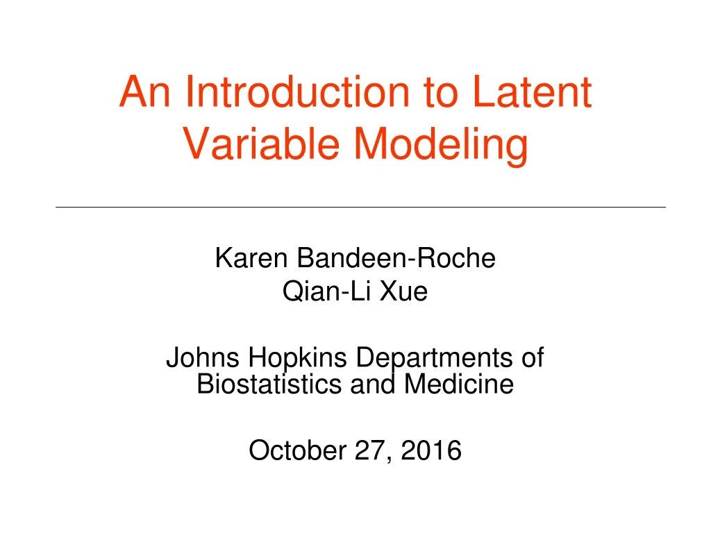
An Introduction to Latent Variable Modeling. Karen Bandeen-Roche Qian-Li Xue Johns Hopkins Departments of Biostatistics and Medicine October 27, 2016. Objectives. What is a latent variable (LV)? What are some common LV models? What are major features of LV modeling?

E N D
An Introduction to Latent Variable Modeling Karen Bandeen-Roche Qian-Li Xue Johns Hopkins Departments of Biostatistics and Medicine October 27, 2016
Objectives • What is a latent variable (LV)? • What are some common LV models? • What are major features of LV modeling? • Hierarchical: structural and measurement components • Fitting • Evaluating fit • Predictions • Identifiability • Why should I consider using—or decide against using—LV models?
Part I: Overview
“LATENT”? • Present or potential but not evident or active: latent talent. • Pathology. In dormant or hidden stage: a latent infection. • Biology. Undeveloped, but capable of normal growth under the proper conditions: a latent bud. • Psychology. Present and accessible in the unconscious mind, but not consciously expressed. The American Heritage Dictionary of English Language, Fourth Edition, 2000 “existing in hidden or dormant form but usually capable of being brought to light” Merriam-Webster’s Dictionary of Law, 1996
“LATENT” • “…concepts in their purest form… unobserved or unmeasured … hypothetical” Bollen KA, Structural Equations with Latent Variables, p. 11, 1989 • “…in principle or practice, cannot be observed” Bartholomew DJ, The Statistical Approach to Social Measurement, p. 12 • “Underlying: not directly measurable. Existing in hidden form but usually capable of being measured indirectly by observables.” Bandeen-Roche K, Synthesis, 2006
“LATENT VARIABLES”? • Ordinary linear regression model: Yi = outcome (measured) Xi = covariate vector (measured) εi = residual (unobserved) Yi = XiTβ+εi
ε . Ordinary Linear RegressionResidual as Latent Variable Yi = XiTβ+εi . Y . ε X Y . . 1 . . . . . . . . . . Boxes denote observables Ovals denote “unobserved” Straight arrows are causal Curved arrows denote association X
Mixed effect / Multi-level modelsRandom effects as Latent Variables . . . β0 + β1 . . . . . vital . . . β2+ β3 . . . . . . β0 . . . . . . non-vital . . β2 . . . time 0
Mixed effect / Multi-level modelsRandom effects as Latent Variables • b0i = random intercept b2i = random slope (could define more) • Population heterogeneity captured by spread in intercepts, slopes +b0i slope: -|b2i| . . . β0 + β1 . . . . . vital . . . β2+ β3 . . . . . . β0 . . . . . . non-vital . . β2 . . . time 0
Mixed effect / Multi-level modelsRandom effects as Latent Variables +b0i slope: -|b2i| . . . β0 + β1 . . . . . vital . . ε . β2+ β3 X Y . . . 1 . . . β0 . . . . b 1 . t . non-vital . . β2 . . . time 0
Latent variable model ε1 δ1 1 1 X1 Y1 Inflammation … Mobility … ξ η 1 ζ1 Xp YM 1 1 δp εM
Latent Variables: What?Integrands in a hierarchical model • Observed variables (i=1,…,n): Yi=M-variate; xi=P-variate • Focus: response (Y) distribution = GYx(y/x) ; x-dependence • Model: • Yi generated from latent (underlying) Ui: (Measurement) • Focus on distribution, regression re Ui: (Structural) • Overall, hierarchical model:
Latent variable model ε1 δ1 X1 Y1 Inflammation … Mobility … ξ η ζ1 Xp YM δp εM Structural Measurement Measurement
Well-used latent variable models General software: MPlus, Latent Gold, WinBugs (Bayesian), NLMIXED (SAS) gllamm (Stata)
Why do people use latent variable models? • The complexity of my problem demands it • NIH wants me to be sophisticated • Reveal underlying truth (e.g. “discover” latent types) • Operationalize and test theory • Sensitivity analyses • Acknowledge, study issues with measurement; correct attenuation; etc.
Latent Variable Models: Philosophy • Why? • To operationalize / test theory • To learn about measurement errors, differential reporting • They summarize multiple measures parsimoniously • To describe population heterogeneity • Popperian learning • Why not? • Their modeling assumptions may determine scientific conclusions • Their interpretation may be ambiguous • Nature of latent variables? • Uniqueness (identifiability) • What if very different models fit comparably? (estimability) • Seeing is believing • Import: They are widely used
Part II: Major elements of latent variable modeling
ExamplePro-inflammation in Older Adults • Inflammation: central in cellular repair • Hypothesis: dysregulation=key in accel. aging • Muscle wasting (Ferrucci et al., JAGS 50:1947-54; Cappola et al, J Clin Endocrinol Metab 88:2019-25) • Receptor inhibition: erythropoetin production / anemia (Ershler, JAGS 51:S18-21) up-regulation Stimulus (e.g. muscle damage) IL-1# TNF-α IL-6 CRP inhibition # Difficult to measure. IL-1RA = proxy
ExamplePro-inflammation in Older Adults Measurement Theory informs relations (arrows) e1 ς Y1 λ1 Inflam. regulation … Adverse outcomes ep Yp λp Determinants Structural
Pro-inflammation in Older AdultsInCHIANTI data (Ferrucci et al., JAGS, 48:1618-25) • LV method: factor analysis model • Continuous indicators, latent variables • Two distinct underlying variables • Down-regulation IL-1RA path=0 • (Conditional independence) IL-6 IL-1RA Inflammation 1 Up-reg. Inflammation 2 Down-reg. CRP IL-18 TNFα
“LATENT VARIABLES”? Linear structural equations model with latent variables (LISREL): Yij = outcome (jth measurement per “person” i) xij =covariate vector (corresponds to jth measurement, person i) λyj =outcome“loading” (relates outcome LV to Y measurement) ηi = latent outcome=random coefficient vector, person i λxj= covariate "loading" (relates covariate LV to jth x measurement) ξi = latent covariate = random coefficient vector, person i εij = observed response residual δij = observed covariate residual ςi = latent response residual vector (specified distribution) Yij = λyjTηi + εij Xij= λjXTξi + δij ηi = Bηi + Γξi + ςi
Latent variable modelsFactor Analysis Measurement Model X=Λxξ+δ Φ=Var(ξ); Θδ=Var(δ)
Latent variable modelsFactor Analysis Measurement Model X=Λxξ+δ Φ=Var(ξ); Θδ=Var(δ) • Assumptions • Most frequently: (ξ, δ) ~ multivariate normal • ξ δ • Constraints on ϕ, Θδ (“theory”) • Ex: Θδ diagonal – indicators uncorrelated given LVs i.e. factor model; conditional independence π
Estimation Overview • Most common: Likelihood-based approaches • Primary challenge: the integral • Approximation (Laplace) • Numerical integration • Stochastic integration • Gradient methods • E-M algorithm • Bayesian approaches (MCMC) • Least squares or analogs
ML EstimationFactor model • Likelihood has closed form (MVN)
Pro-inflammation in Older Adults(Bandeen-Roche et al., Rejuv Res) • LV method: factor analysis model .36 -.59 IL-6 . 59 IL-1RA -.40 . 45 Inflammation 1 Up-reg. Inflammation 2 Down-reg. CRP . 31 IL-18 .20 . 31 TNFα
MethodsGlobal measures • Goodness of fit testing • Hypothesis: H0: GY|X(y|x) = FY|X(y|x;π,β) for some (π,β) εΘ • Method: Deviance goodness of fit testing, analogs • Usual issues for quality of asymptotic distribution approximation • Inflammatory analysis: Deviance goodness of fit pvalue > 0.5 • Global fit indices: “Hundreds” of them
MethodsResidual checking • Per-item: Observed – expected • Residuals with respect to association structure • Continuous Y: Covariance or correlation matrix residuals S- • Categorical Y: • Odds ratio matrix residuals: Q- Implied, Q has elements [ad/bc]ij from cross-tabulation of items i & j • O-E cell counts for the full cross-tabulation of items (I1xI2x…xIM cells, where Ij denotes the number of categories for item j) • All cases: normalized residuals most useful
ExampleResidual checking • NFΚB-gated systemic inflammation
MethodsOther • Posterior predictive checking Gelman et al., Statistica Sinica, 1996 • Pseudo-value analysis: More to come
Latent variable scoringOverview • Task: Estimate persons’ underlying status • “fill in” values for the Ui • Fundamental tool: Posterior distribution
Latent variable scoringPosterior mean estimation • Posterior mean = most common method • Typically: Empirical Bayes (filling in estimates for parameters) • Minimizes expected posterior quadratic loss • Linear case (LISREL): Yields Best Unbiased Linear Predictor (BLUP)
Latent variable scoringLISREL (factor) measurement model • Posterior mean is closed form linear , • “Regression method” Σ= Var(X)
Latent variable scoringLISREL (factor) measurement model • Alternative method: “Bartlett” scores • Paradigm: treat ξi as fixed parameters per i; estimate these via weighted least squares δi ~ N(0, ) • Which is better? • Depends on analytic purpose
Latent variable scoringFrequent purpose: “multi-stage” regression • Step 1: Fit full latent variable measurement model(s) (Y,X) , • Step 2:Obtain predictions Oi given Yi, and/or Xi, • Step 3: Obtain via regression of Oi on Xi or Yi on Oi, as case may be
Latent variable scoringFrequent purpose: “multi-stage” regression • Result: In the fully linear model, provided that estimators in Step 1 are consistent: • (a) When the covariate is being predicted, employing the regression method in Steps 2-3 consistently estimates B • (b) When the outcome is being predicted, employing the least squares method in Steps 2-3 consistently estimates B • Brief rationale for (a): method is analogous to regression calibration with replicates Carroll & Stefanski, JASA, 1990
One last issueIdentifiability • Models can be too big / complex • A model is non-identifiable if distinct parameterizations lead to identical data distributions • i.e. analysis not grounded in data • Weak identifiability is common too: • Analysis only indirectly grounded in data (via the model)
Identifiability strong model analysis data (ground)
Identifiability weak model analysis data (ground)
Identifiability non model analysis data (ground)
Objectives • What is a latent variable (LV)? • What are some common LV models? • What are major features of LV modeling? • Hierarchical: structural and measurement components • Fitting • Evaluating fit • Predictions • Identifiability • Why should I consider using—or decide against using—LV models?