Download
1 / 14
140 likes | 366 Views
Latent variable models for time-to-event data. A joint presentation by Katherine Masyn & Klaus Larsen UCLA PSMG Meeting, 2/13/2002. Overview. 1) Introduction to survival data 2) Discrete-time survival mixture analysis (Katherine) 3) Latent variable models for (continuous)

E N D
Latent variable models for time-to-event data A joint presentation by Katherine Masyn & Klaus Larsen UCLA PSMG Meeting, 2/13/2002
Overview 1) Introduction to survival data 2) Discrete-time survival mixture analysis (Katherine) 3) Latent variable models for (continuous) time-to-event data (Klaus) 4) Extensions
Time-to-event Data A record of when events occur (relative to some “beginning”) for a sample of individuals For example, time from sero-conversion to death in HIV/AIDS patients, age of first alcohol use in school-aged children, time to heroine use following completion of methadone treatment
Methods for this type of data must consider an important feature, known as censoring: The event is not observed for all subjects Methods must also handle covariates that may change with time, e.g., CD4 count Data: Time (interval) of event or censoring, indicator for whether or not the event occurred, and relevant covariates
Discrete vs. Continuous Time Continuous: The “exact” time of an event (or censoring) for each subject is known, e.g., time of death Discrete: The time of an event (or censoring) for each subject is only recorded for an interval of time, e.g., grade of school drop out
Discrete-Time Survival Mixture Analysis (DTSMA) Katherine Masyn, UCLA Based on the work of Muthén and Masyn (2001) and Masyn (2002) Research supported under grants from NIAAA, NIMH, NIDA, and in collaboration with Bill Fals-Stewart at the Research Institute for Addictions at SUNY-Buffalo
Let T be the time interval in which the event occurs: T = 1, 2, 3,... S(t), called the survival probability, is defined as the probability of “surviving” beyond time interval t, i.e., the probability that the event occurs after interval t: S(t) = P(T > t) h(t), called the hazard probability, is defined as the probability of the event occurring in the time interval t, provided it has not occurred prior to t: h(t) = P(T = t | T t)
Hazard Probability Plot Survival Probability Plot
x1 x2 xJ u2 uJ u1 . . . C Z DTSMA with Covariates
GGMM + DTSMA UM+1 UM+2 UM+3 UM+J . . . z C i s Y1 Y2 Y3 YM . . .