Download
1 / 28
320 likes | 648 Views
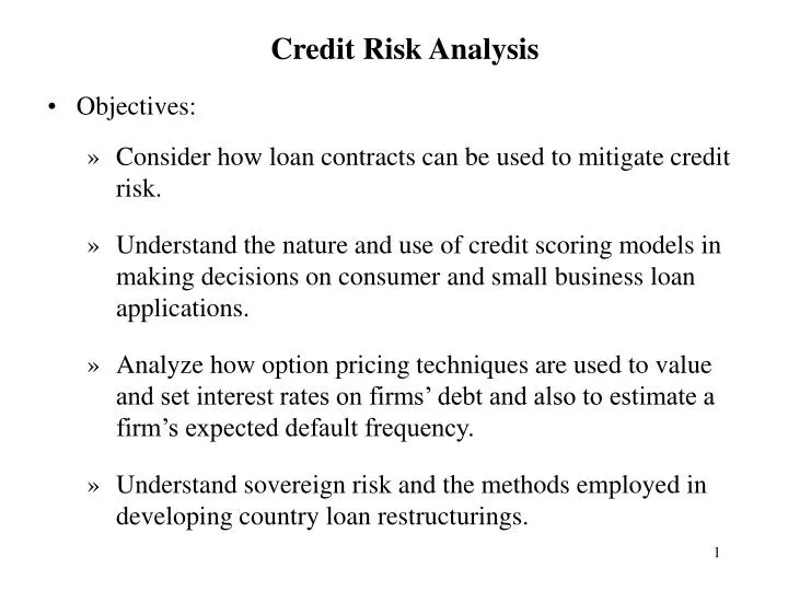
Credit Risk Analysis. Objectives: Consider how loan contracts can be used to mitigate credit risk. Understand the nature and use of credit scoring models in making decisions on consumer and small business loan applications.

E N D
Credit Risk Analysis • Objectives: • Consider how loan contracts can be used to mitigate credit risk. • Understand the nature and use of credit scoring models in making decisions on consumer and small business loan applications. • Analyze how option pricing techniques are used to value and set interest rates on firms’ debt and also to estimate a firm’s expected default frequency. • Understand sovereign risk and the methods employed in developing country loan restructurings.
Controlling Credit Risk with Loan Contracts • Loans are usually classified into different types: • Commercial and Industrial (C&I) Loans: loans to large and small businesses. May be secured (collateralized) or unsecured, term loans or lines of credit. • Sovereign Loans: Loans made to foreign governments, usually in the form of syndicated loans made by large, multi-national FIs. • Consumer Loans: Loans to individuals, including installment loans (e.g., auto loans) and unsecured revolving lines of credit (e.g., credit card debt). • Real Estate Loans: Commercial and residential mortgages. • Other: Include agricultural loans and loans to municipal governments.
All of the previous types of loans are subject to default (credit) risk. Whether or not a lender (e.g., commercial bank or finance company) decides to extend credit depends not only on the potential borrower’s risk but also on the • terms of the loan • lender’s ability to monitor the borrower • lender’s ability to enforcerestrictions on the borrower • These determinants of credit risk depend on the legal provisions of the loan contract. • Let us outline the typical parts of a C&I loan agreement and consider how the contract provisions help to control credit risk. (See sample Business Loan Agreement for a line of credit made by Bank of America to Leapfrog Enterprises.)
Terms of the Loan • Principal: Amount or maximum amount of the loan. CR • Maturity: longer maturities CR • Take-down schedule: timetable for withdrawing funds • Interest rate: fixed or floating. Floating rates may be tied to the Prime Rate or LIBOR. The borrower’s spread over the base rate may vary with the borrower’s current financial condition (e.g., leverage). Higher spreads provide protection against default but can CR. • Pre-payment provisions and unused commitment fees: affects interest rate risk for fixed-rate loans. • Warranties • Borrower guarantees financial statements are accurate • Borrower has good title to assets • Borrower is complying with law and not involved in litigation. • Borrower has filed for and paid required taxes.
Covenants • Positive covenants: Actions a borrower agrees to take. • Periodically furnish financial information to lender. • Permit lender to audit any of the firm’s records. • Promptly advise lender of changes in management or any event that materially effects the firm’s financial condition. • Maintain insurance on specified assets. • Maintain certain balance sheet and income statement ratios. • Use all loan proceeds for specified purpose and conduct business in the same manner as is now carried on. • Negative covenants: Actions borrower agrees not to take. • Taking on additional debt or pledging its assets to creditors. • Repaying loans from owners or shareholders. • Merging with any other business. • Limits on payment of dividends and manager compensation. • Selling assets/property except in normal course of business.
Other Requirements • Specific assets may be assigned as collateral. • Specifying which state law governs the agreement. • Specifying how disputes will be settled (e.g., arbitration). • Events of Default • Failure to make any principal or interest payment, abide by any covenant, default on any other debt obligation, or file for bankruptcy triggers default on the loan. • Lender can then demand that any remaining principal and unpaid interest will become immediately due. • Lender can then sell any collateral and apply the proceeds to payment of the loan. • In summary, the contract contains numerous provisions whose purpose is to protect the lender’s extension of credit.
Credit Scoring Models • Credit scoring models have been most often used in consumer lending but, increasingly, are being used in small business lending, especially by large FI lenders. • Credit scoring models use historical data on loan defaults or business bankruptcies to predict the likelihood of default for new loan applicants. The models’ results can be used to • Decide whether a loan request should be approved. • Decide the terms of a loan: maximum amount lent (credit limit) and interest rate (credit spread). • The benefits of credit scoring models are • Provide a rigorous, objective method for using financial data to screen the credit of loan applicants. • Reduces lenders’ time and cost of making loan decisions.
Altman’s Z-Score Model: uses a statistical technique, Multiple Discriminant Analysis (also could use logit or probit analysis) to classify firms into those likely to become bankrupt or non-bankrupt over a given future horizon. • Past financial data on firm financial ratios and bankruptcies were used to estimate the regression equation • where • Z = 0 if firm becomes bankrupt and = 1 if firm does not. • X1=Working Capital / Total Assets • X2=Retained Earnings / Total Assets • X3=EBIT / Total Assets • X4=Market Value of Equity / Book Value Long-Term Debt • X5=Sales / Total Assets
The higher is Z, the lower is the firm’s estimated risk of bankruptcy. • For a given Type I error (classifying firm as not bankrupt when it is) and a given Type II error (classifying a firm as bankrupt when it is not), a critical value of Z could be used to approve or deny a loan. For example: • If Z 2.675 assign to non-bankrupt group and approve loan • If Z < 2.675 assign to bankrupt group and deny loan. • Consumer Credit Scoring Models: models use data on historical loan defaults to statistically determine the most relevant information for predicting defaults on credit cards, auto loans, mortgages, and other consumer credit. • Model information must comply with Federal Reserve Reg. B relating to the Equal Credit Opportunity Act of 1974.
Regulation B states that applicant characteristics included in a credit score must be “demonstrably and statistically sound.” It prohibits certain information, such as race, whether the applicant has a telephone, etc. • Other information must be statistically justified and its soundness systematically reviewed and updated. Examples: late payments, amount of time credit has been established, credit taken relative to credit limit, length of time at current residence, employment history, history of bankruptcies or collections. • Individual lenders may develop their own “in-house” credit scoring model for particular types of loans. • Alternatively, lenders buy credit scoring models. A popular one is the FICO model sold by Fair Isaac & Co. For an estimate of your FICO score, see www.bankrate.com/brm/fico/calc.asp.
Option Models of Firm Default Risk • Fischer Black, Myron Scholes, and Robert Merton, the developers of modern option pricing models, recognized that option pricing methods can be used to value a firm’s default-risky debt, such as a bond or loan. • Not only can option pricing value (price) debt that may default, it can be used to estimate the fair interest rate (credit risk premium) to charge on a business loan. It also can be used to estimate the probability of default. • KMV, a subsidiary of Moody’s uses this option approach to calculate an actual firm’s default probability, which it calls “expected default frequency” or EDF. It sells EDFs for individual firms, which is a measure of credit risk that is an alternative to Moody’s and S&P’s credit ratings.
To illustrate the option approach, consider the following simple example. Suppose a firm has assets whose value currently equals $ A, but that are risky and change randomly over time. • The firm is assumed to have a simple capital structure. It has a single ZCB or loan outstanding that matures in T years and promises to pay $B at maturity. The rest of its financing comes from shareholders’ equity. It is assumed to issue no new securities until possibly after date T. • If we let D denote the current market value (price) of this firm’s debt or bonds and let E be the current market value of its shareholders’ equity, then the market value of the firm’s assets must equal the total value of the firm’s liabilities or contingent claims on these assets: A = D + E
Firm Balance Sheet Assets Liabilities A = value of risky assets D = value of debt = value of promised payment of B in T years. E = value of shareholders’ equity • While the sum, D+E, can be deduced from the value of A, • we would like to determine the individual values of D and E.
To do this, consider the value of the firm’s debt and equity, • in relation to the firm’s assets, at date T when the debt matures. • Let AT, DT, andET denote the values of the firm’s assets, debt, • and equity at date T. • Because the firm’s assets are risky, their value at date T could • be insufficient to pay the promised value of the firm’s debt, B. • If so, it is assumed that the firm is bankrupt and shareholders’ • equity becomes worthless (ET = 0). The value of debt then • equals the value of the firm’s assets (DT = AT ). • If, instead, the value of the firm’s assets at date T are • sufficient to pay the promised value of the firm’s debt, then • the debt’s value at maturity equals its promised payment • (DT = B). In this case, the value of equity equals the residual • asset value (ET = AT - B).
Value of Debt and Equity at Date T Value Debt, DT B Equity, ET 0 0 B Date T Firm Asset Value, AT
Thus, considering both the bankruptcy and no-bankruptcy • cases, the date T values of debt and equity can be written as: DT = min[ B, AT ] = B - max[B - AT , 0 ] ET = max[ AT - B, 0 ] • We can now apply insights from option pricing. The value of • equity is analogous to the payoff of a call option written on the • firm’s assets and having an exercise price equal to B. • The value of debt equals the promised payment, B, less the • value of a put option written on the firm’s assets and having • and exercise price equal to B.
Hence, using an option pricing formula, such as the Black- • Scholes formula, would allow us to solve for the current values • of the firm’s equity and debt. • For example, if r is the continuously-compounded risk-free • (default-free) interest rate and is the standard deviation of the • return on the firm’s assets, then the current value of equity is:
Since D = A- E, the value of debt is then determined: • Also, once the current market value of debt is known, the • debt’s (continuously-compounded) promised yield to maturity, • which we denote as R, can be computed: • Furthermore, it can be shown that an estimate of the firm’s • probability of default or EDF is 1 – N(d2) = N(-d2)
Example: Calculate the fair (break-even) interest rate a bank would need to charge on the following firm’s loan: • Loan has a T=2 year maturity with no interim payments. • Promised payment at maturity (principal+interest) is B=$4 m. • Bank’s continuously-compounded marginal cost of funds for this two-year maturity is r = 7.00 % • Current value of the firm’s assets backing the loan is A=$7m. • Annualized variance of the return on the assets is2 = 20%. • Using these values, we find d1 =1.42 and d2 =0.79. Thus N(0.79) = 0.78 and N(-1.42)=1-N(1.42) = 1-0.92 = 0.08. Hence, the firm’s EDF = 1- N(d2) = 1 – 0.78 = 22% and its debt’s value and fair loan rate is
Hence, we see that the firm’s fair default risk premium is R – r = 10 % - 7 % = 3 %. • To implement this option pricing approach, estimates of the market value of a firm’s assets, A, and the volatility of the return on these assets,, are needed. • For a firm that has publicly traded shareholder’s equity, the value of A and can be estimated using the firm’s market value of common stock, E, as well as its stock’s volatility. This is done using the previously given formula
One additional insight is worth noting. If this firm’s debt • (bonds or loans) were insured against default by an insurance • company’s guarantee or a bank’s letter of credit, then value of risky debt + value of guarantee = value of default-free debt or value of risky debt = value of default-free debt - value of guarantee • Since we showed that DT = B - max[B - AT , 0 ], this confirms • that at maturity the firm’s default-risky debt equals the payoff • of risk-free debt, B, less value of a guarantee, max[B - AT , 0 ]. • Thus, the current value of a debt guarantee, G, equals the value • of a put option on the firm’s assets with an exercise price of B:
Developing Country Loans and Sovereign Risk • If lesser developed countries (LDCs) have low domestic savings but profitable investments, one expects them to run current account deficits and seek financing abroad. • Types of capital inflows: • Bank loans: typically syndicated loans denominated in $ or other reserve currencies. • Bond finance: important until large Latin American defaults during 1930’s. Many former bank loans converted to “Brady” bonds starting in 1989 in exchange for debt relief. • Direct foreign investment: Usually a foreign firm expanding or acquiring a subsidiary in an LDC. Risk of nationalization and repatriation of profits. • Official lending: from IMF or World Bank. Principle of Conditionality: loans tied to macro-economic reform.
LDC loans and bonds differ from domestic C&I loans because of a lack of a bankruptcy process in which lenders can make recoveries following default. • Even if a loan is made to a LDC firm that is creditworthy (solvent), the firm’s ability to repay is often controlled by its government. • In the absence of an international bankruptcy court or “gunboat diplomacy,” a debtor chooses to make payment to avoid various penalties: • Being excluded from future access to capital markets • Trade sanctions or withdrawal of trade credits. • These penalties do not benefit lenders, so it is in the interest of both borrowers and lenders to reach a settlement.
Debt Forgiveness: 1989 proposals by Treasury Secretary Brady restructured LDC bank loans to bonds in return for debt forgiveness. • Because of “debt overhang” a lender may be better-off agreeing to partial debt forgiveness. • Example: A country receives a loan with promised payment of B=100. The country’s resources available to pay the loan are A = 300. Suppose a penalty of P = ½A could be imposed on the LDC if it failed to repay. • Suppose, next, that the country experiences a macro-shock and A falls from 300 to 160. Will it repay its loan of 100? • Note that P = ½A= 80, so the country will repay if B < 80. Lenders will be better off agreeing to this partial forgiveness.
Debt Buybacks: Following economic crisis, the market value of an LDC’s debt falls. Is it worthwhile for the LDC to buy back some of its debt at a discount (e.g., Bolivia in 1980s)? • Example: Suppose an LDC has 10 different loans each with a promised payment of 100, for a total promised payment of B = 1000. The LDC has suffered a severe shock, to that it now has only a 1/5 chance of obtaining 1000 in resources: • Assuming the country repays whenever possible, the market value of the loans (assuming risk-neutrality) is • D = (1/5)1000 = 200 • Thus, the market value of the LDC’s indebtedness is 200.
Suppose that the LDC can impose economic austerity measures to raise 100 (e.g., from the IMF) to buy back ½ of its loans at the market price of 20 per loan. Its remaining promised payment is then 500. The market value of it remaining debt is therefore D = (1/5)500 = 100 and the market value of its profits after (possible) repayment is (1/5)(1000-500) = 100 making its net indebtedness equal to zero. Thus, adding in the 100 buy back cost shows that the debt buyback was worthwhile since 100 + 0 < 200.
However, suppose the LDC had 30 loans (severe debt overhang), each with a promised payment of 100, for a total promised payment of 3000. Given the same resources, would a buyback still be worthwhile? • In this case, the market value of its indebtedness is still • D = (1/5)1000 = 200 • If the LDC uses 100 to buy back ½ of its loans at market prices, its remaining promised payment is then ½(3000) = 1500. • The market value of its remaining debt is still • D = (1/5)1000 = 200 • Thus, the costly 100 debt buyback has done nothing to reduce the market value of its indebtedness and should be avoided.
Debt for Equity Swaps: These were a method of partial forgiveness used by some LDCs. They involve the following steps: • An LDC $-denominated loan is sold to a broker at a discount. • The broker sells this loan to a multi-national firm that wishes to expand (invest) in the LDC. • The multi-national takes the loan to the LDC’s central bank and obtains approval for the new investment. • The central bank gives the multi-national payment in the domestic currency (often at an over-valued exchange rate), which is then used to finance its investment. • These swaps can lead to higher inflation because they expand the domestic money supply.