Download
1 / 29
500 likes | 1.22k Views
Credit Risk – Loan Portfolio and Concentration risk. Class 15; Chap 12. Lecture outline. Purpose: Gain a working knowledge of how FIs measure and manage the risk of a loan portfolio Simple models Migration analysis Concentration limits Modern Portfolio Theory Models

E N D
Credit Risk – Loan Portfolio and Concentration risk Class 15; Chap 12
Lecture outline • Purpose: Gain a working knowledge of how FIs measure and manage the risk of a loan portfolio • Simple models • Migration analysis • Concentration limits • Modern Portfolio Theory Models • Portfolio Diversification • KMV model • Loan Concentration Models • Loan volume-Based Model
Migration Analysis Basic Idea: • FI managers want to know how the credit risk (Rating) of loans in their portfolio should change over time(that is, what can managers expect). • If the actual change is different from what managers expect they can ration credit or adjust premiums For Example: • Suppose that on average over the last five years 11 out of 100 loans have been downgraded from a rating of BBB to a rating of BB each year. • If the FI has a portfolio of 500 BBB rated loans How many loans should the manager expect to be rating of BB by the end of the year? • Suppose that over the last year, on average, 15 out of 100 BBB loans were downgraded to a rating of BB, would the manager be concerned? • This would suggest that BBB rated loans have become riskier – So what can the manager do? • The manager could then cut-back on lending to this rating category or increase the credit risk premium 55 loans should drop to a rating BB Yes! More loans than expected were downgraded
Measuring Rating Migration Loan Rating Migration Matrix • The migration matrix tells us the percentage of bonds that start in one rating category and move to another • We read the table by rows across columns DO NOT READ DOWN THE COLUMNS • The number inside the matrix are called transition probabilities. They tell us what portion of an FIs portfolio is expected to transition to a new rating each year • Example: • Of the loans that started the year in AAA-A category 85% remained in AAA-A 10% transitioned to BBB-B 4% transitioned to CCC-C 1% Defaulted The column header tells us the rating category where bonds end the year The row header tells us the rating category where loans begin the year
Migration Analysis Example Suppose an FI manager has 211 BB rated loans, 310 AA rated loans and 130 C rated loans what would the manager expect his portfolio to look like at the end of the year • Begin with the AA rated Loans • AAA-A = (310)(.91) = 282.1 • BBB-B = (310)(.08) = 24.8 • CCC-C = (310)(.01) = 3.1 • D = (310)(0) = 0 • BB rated Loans • AAA-A = (211)(0.08) = 16.88 • BBB-B = (211)(0.83) = 175.13 • CCC-C = (211)(0.05) = 10.55 • D = (211)(0.04) = 8.44 • Loan Portfolio at the end of the year • AAA-A = 302.88 • BBB-B = 212.93 • CCC-C = 117.65 • D = 17.54 • C rated Loans • AAA-A = (130)(0.03) = 3.9 • BBB-B = (130)(0.10) = 13 • CCC-C = (130)(0.80) = 104 • D = (130)(0.07) = 9.1 Sum each category
Suppose an FI has 100 BBB rated loans, 500 A rated loans, and 13 C rated loans. Calculate the expected loss of the portfolio if all loans have face value of $100,000. The average recovery rate for loans is 60%. The transition matrix is shown below Step #1 – calculate the number of bonds in each category expected to fail AAA-A 500*.02 = 10 BBB-B 100*.04=4 CCC-C 13*.06 = .78 Step #2 – calculate the loss on the portfolio AAA-A 10*100,000*0.6 = 600,000 BBB-B 4*100,000*0.6 = 240,000 CCC-C 0.78*100,000*0.6 = 46,800 Total $886,800.00
Concentration Limits Basic Idea: The FI can set limits on the amount lent to an individual borrower or a sector to limit exposure to a particular borrower or sector • If defaults of a borrower/sector are highly correlated the FI will usually set one combine limit • Geographic limits are also commonly used • Regulators have limited the amount lent to one borrower to 10% of equity capital
Concentration limits Example Suppose management has placed a limit on lending to the auto manufacturing sector such that the maximum potential loss is no greater than 10% of equity capital. The firm has total assets of 500 mill and liabilities of 450 mill. Historical recovery from the Auto manufacturing sector is 40%. How much can the FI lend to the auto manufacturing sector? Step #1 calculate the maximum equity capital the firm can lose If the full amount lent to auto manufactures (X) defaults the FI will lose 1-.4= 60% of the principal lent Step #2 Calculate the loan principal that can be lent to auto manufactures Loan concentration limit The maximum amount the FI can lend to auto manufactures
Example: Managers at Manhattan bank have limited lending to the computer software sector. No more than 5% of total loan value can be lent to this sector. The bank is currently at its limit. How much software loan value will the bank have to sell if the value of their loan portfolio decreases by 20% but the value of their software loans stays constant. Assume that the loan portfolio currently has a value of $50M. Step #1 calculate the maximum equity capital the firm can lose Step #2 Calculate the loan principal that can be lent to auto manufactures X ≤33.333%
Portfolio Diversification Basic Idea: • FIs can reduce the level of loan portfolio risk by ensuring that the portfolio is well diversified – changes in default probabilities are not perfectly correlated. • The portfolio diversification model also allows the manager to measure the level of risk in his/her portfolio • The portfolio diversification model also allows FI managers to measure how well their portfolio is performing relative to other allocations (portfolios) with the same risk level
Portfolio Diversification- Risk and Return Expected Return of a portfolio: • Given historical returns of the individual assets, how do you calculate the expected portfolio return? • It is just the weighted average of individual returns Risk of a Portfolio: • Risk is measured by the volatility (standard deviation) of portfolio returns • This can be calculated using the variance of individual asset returns
Portfolio Diversification – Example 2 Loan Portfolio: Given the following statistics for two loans, find the risk and return of the portfolio Step #1 Calculate the portfolio expected return Step #2 Calculate the risk (volatility) of the portfolio
Portfolio Diversification – Example Portfolio Performance (Side Note): • The question here is can portfolio manager do better with a different allocation? • The answer is maybe – in the 2 asset case NO (if there are only 2 assets in the universe )
Example: Suppose an FI holds a bond portfolio that is fully invested in two sectors: $20 million to consumer durables and $50 million to the healthcare sector. The expected return and volatility for the consumer durables sector portfolio is .125 p.a. and .081 p.a. respectively. The expected return and volatility for the health care sector portfolio is .083 p.a. and .041 p.a. respectively. Find the risk and return of the portfolio. Correlation between the two portfolios is .32
Moody’s KMV Model Basic Idea: • Diversification models are only appropriate for assets with normally distributed returns but bond & loan returns are not usually considered normal • Loans are also infrequently traded – this makes estimating the expected return and standard deviation from market data very difficult • The Moody’s KMV portfolio manager model addresses these shortcomings • Main contribution – they use proprietary probabilities of default (EDF) to directly estimate the return on the loan and use that return in the portfolio diversification model • We add one more step
Moody’s KMV – Loan Risk & Return Loan Returns: All-in-spread AIS = (return on loan – funding cost) + annual fees Expected default frequency EDF = probability of default Loan Risk: Correlation: In the KMV model the correlation is the correlation between the systematic component of a bank asset returns (e.g. the systematic component of loan 1 and loan 2 returns) The return on the loan i.e. “k” Volatility of the company’s EDF
Moody’s KMV Model – Example Given the following portfolio of loans calculate the risk and return of the portfolio Step #1 Calculate Expected Loan Returns for each loan
Moody’s KMV Model – Example Given the following portfolio of loans calculate the risk and return of the portfolio Step #2 Calculate Loan Risk (volatility) - for each loan
Moody’s KMV Model – Example Given the following portfolio of loans calculate the risk and return of the portfolio Step #3 Calculate the portfolio return
Moody’s KMV Model – Example Given the following portfolio of loans calculate the risk and return of the portfolio Step #4 Calculate the risk (volatility) of the portfolio Portfolio Risk = 2.52% Portfolio return = 5.99%
Loan #1 EDF = 0.05 LGD = 0.30 AIS = 0.12 Principal = 25 mill Loan #2 EDF = 0.07 LGD = 0.60 AIS = 0.20 Principal = 75 mill Example: Suppose an FI has holds 2 loans in its portfolio with the given characteristics. Find the portfolio return if the correlation between the two firms assets is 0.45
Loan Volume-Based Model Basic Idea: • Loan prices are difficult to obtain but volume (aggregate principal) is available • The volume based model measures how different a bank’s lending activity is from the average bank in a pier group
Loan Volume-Based Model - Example Given the concentration of lending to each of the four sectors for bank A and bank B along with the national average below, which of the two bank differs more in its lending activity from the average national bank Step #1 Calculate the squared difference between the national average and each bank Bank A Bank B
Loan Volume-Based Model - Example Given the concentration of lending to each of the four sectors for bank A and bank B along with the national average below, which of the two bank differs more in its lending activity from the average national bank Step #2 average the squared differences and take the square root Bank A Bank B
Loan Volume-Based Model - Example Given the concentration of lending to each of the four sectors for bank A and bank B along with the national average below, which of the two bank differs more in its lending activity from the average national bank Is it bad to be different? • Banks may specialize in certain types of lending • Banks may be located in a region where certain types of lending is more prevalent
Lecture Summary • We saw 5 different ways to measure the credit risk of a portfolio of assets • Simple models • Migration analysis • Concentration limits • Modern Portfolio Theory Models • Portfolio Diversification • KMV model • Loan Concentration Models • Loan volume-Based Model