Download
1 / 36
390 likes | 543 Views
Structure from Motion. ECE 847: Digital Image Processing. Stan Birchfield Clemson University. Acknowledgment. Many slides are courtesy of others. SVD. Any mxn matrix A can be decomposed as where This is the singular value decomposition (SVD). mxm. mxn. nxn. =.

E N D
Structure from Motion ECE 847:Digital Image Processing Stan Birchfield Clemson University
Acknowledgment Many slides are courtesy of others
SVD • Any mxn matrix A can be decomposed as • where • This is the singular value decomposition (SVD) mxm mxn nxn
= Tall and short matrices Tall matrix m>n, p = n mxm mxn nxn m<n, p = m Short matrix = mxm mxn nxn
Compact version Tall matrix Tall matrix m>n, p = n = mxm mxn nxn m<n, p = m Short matrix Short matrix = mxm mxn nxn
Compact version (cont.) Tall matrix Tall matrix m>n, p = n = mxn nxn nxn m<n, p = m Short matrix Short matrix = mxm mxm mxn
SVD reveals structure • Let r be the index of the smallest non-zero singular value • Then • Easy to show:
Eigen / singular • Singular values and singular vectorswork likeeigenvalues and eigenvectors: • First p eigenvalues of ATA (or AAT) are squares of the singular values of A:
Condition number • A is non-singular if and only if • In real life, matrices are never singular. • The condition number of A is • If 1/C is near the machine’s precision, then A is ill-conditioned. It is dangerous to invert A.
Norms Singular values readily yield norms: • Induced Euclidean norm: • Frobenius norm:(Euclidean norm, treating matrix as vector)
Least squares where The set of equations is solved as or
Least squares (cont.) • Minimum norm least squares solution to Ax=b, i.e., the shortest vector x that achieves is unique and is given by • where pseudoinverse inverts all nonzero singular values
Homogeneous system • What if b is all zeros? • Then the minimum-norm solution is not interesting, b/c it will be x=0 always • Instead, find unit-norm solution • Solution is given by (the right singular vector associated with the smallest singular value)
Enforcing constraints Find closest matrix to A in the sense of Frobenius norm that satisfies constraints exactly: • Factorize A = USVT • Change S to S’ to satisfy constraints • Put back together: A’ = US’VT Example: Enforce rank of A by setting small singular values to zero
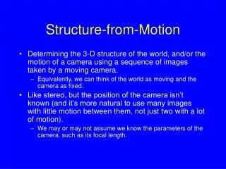
Structure from motion • Structure from motion (SFM) recovers • scene geometry • camera motion from a sequence of images • Could be called structure (or shape) and motion from video (SAMV), but nobody does this
SFM preliminaries • Collect F frames of P points (with correspondence) • Camera coordinate system: centered at focal point and aligned with image axes (x and y in image, positive z along optical axis) • World coordinate system is coincident with first camera (arbitrary)
SFM under perspective projection pth point xp-tf xp • Perspective imaging: • Equation counting: • 2FP+1 equations (extra equation from scale ambiguity) • 3P + 6(F-1) unknowns • Required:2FP+1 >= 3P + 6(F-1)With 2 frames, need at least 5 points if fth camera coord sys. tf world coord sys. jf
Perspective: 2 frames of 5 points • Show graphically that with fewer than 5 points, there is always wiggle room between camera frames
8-point algorithm • Longuet-Higgins • Hartley normalization
SFM under orthographic projection • Orthographic imaging ignores depth: • Equation counting: • 2FP+F equations (extra eqn. for each frame: set z motion to 0) • 3P + 6(F-1) unknowns (same as perspective) • But equations are not independent (complicated proof omitted) • 2 frames is not enough • With 3 frames, need at least 4 points
Orthography: 3 frames of 4 points • Show graphically the wiggle room with < 3 frames or < 4 points
Factorization rotation • Recall: • Stack into measurement matrix: 4xP 2FxP 2Fx4 (Tomasi and Kanade 1992) measurement = motion x shape
Subtracting centroid • Place world origin at centroid of points: • Then subtract centroid of image coordinates per frame:
Registered measurements • This leads to the registered measurement matrix: 3xP 2FxP 2Fx3 registered measurement = rotation x shape
3 3 0 3 0 0 Rank theorem • Similarly, • Use SVD to enforce rank constraint: • This reduces effects of noise in a robust, stable way
Euclidean constraints • But our choice was arbitrary • Solution is unique only up to affine transformation • Impose metric constraints to solve for Q: for any invertible 3x3 matrix Q use least squares, then Cholesky decomposition
Algorithm summary Tomasi-Kanade factorization for SFM: (Quadratic equations require nonlinear minimization)
Handling occlusion Unknown image measurement pair (ufp,vfp) in frame f can be reconstructed if • p is visible in 3 image frames • 3 other points are visible in 4 frames
Occlusion results ping pong ball rotated 450 degrees 84% of data hallucinated from 16%
Factorization extensions • Poelman and Kanade (1994): Paraperspective • Costeira and Kanade (1995): Multibody factorization • Sturm and Triggs (1996): Perspective, fixed rank algorithm to speed computation multibody (Costeira and Kanade) results
Planar parallax • See Irani
Using dynamics • We have looked at batch methods. Now incremental methods. • A. Davison real-time reconstruction
Texture mapping Depth image Texture image Triangle mesh • Pollefeys Textured 3D Wireframe model