Download
1 / 43
430 likes | 595 Views
11/18/11. Structure from Motion. Computer Vision CS 143, Brown James Hays. Many slides adapted from Derek Hoiem , Lana Lazebnik , Silvio Saverese , Steve Seitz, and Martial Hebert. This class: structure from motion. Recap of epipolar geometry Depth from two views

E N D
11/18/11 Structure from Motion Computer Vision CS 143, Brown James Hays Many slides adapted from Derek Hoiem, Lana Lazebnik, SilvioSaverese, Steve Seitz, and Martial Hebert
This class: structure from motion • Recap of epipolar geometry • Depth from two views • Affine structure from motion
Recap: Epipoles • Point x in left image corresponds to epipolar line l’ in right image • Epipolar line passes through the epipole (the intersection of the cameras’ baseline with the image plane
Recap: Fundamental Matrix • Fundamental matrix maps from a point in one image to a line in the other • If x and x’ correspond to the same 3d point X:
Structure from motion • Given a set of corresponding points in two or more images, compute the camera parameters and the 3D point coordinates ? ? Camera 1 ? Camera 3 ? Camera 2 R1,t1 R3,t3 R2,t2 Slide credit: Noah Snavely
Structure from motion ambiguity • If we scale the entire scene by some factor k and, at the same time, scale the camera matrices by the factor of 1/k, the projections of the scene points in the image remain exactly the same: • It is impossible to recover the absolute scale of the scene!
Structure from motion ambiguity • If we scale the entire scene by some factor k and, at the same time, scale the camera matrices by the factor of 1/k, the projections of the scene points in the image remain exactly the same • More generally: if we transform the scene using a transformation Q and apply the inverse transformation to the camera matrices, then the images do not change
Projective structure from motion Xj x1j x3j x2j P1 P3 P2 • Given: m images of n fixed 3D points • xij = Pi Xj, i = 1,… , m, j = 1, … , n • Problem: estimate m projection matrices Pi and n 3D points Xj from the mn corresponding points xij Slides from Lana Lazebnik
Projective structure from motion • Given: m images of n fixed 3D points • xij = Pi Xj, i = 1,… , m, j = 1, … , n • Problem: estimate m projection matrices Pi and n 3D points Xj from the mn corresponding points xij • With no calibration info, cameras and points can only be recovered up to a 4x4 projective transformation Q: • X → QX, P → PQ-1 • We can solve for structure and motion when • 2mn >= 11m +3n – 15 • For two cameras, at least 7 points are needed
Types of ambiguity • With no constraints on the camera calibration matrix or on the scene, we get a projective reconstruction • Need additional information to upgrade the reconstruction to affine, similarity, or Euclidean Projective 15dof Preserves intersection and tangency Preserves parallellism, volume ratios Affine 12dof Similarity 7dof Preserves angles, ratios of length Euclidean 6dof Preserves angles, lengths
Affine ambiguity Affine
Bundle adjustment • Non-linear method for refining structure and motion • Minimizing reprojection error Xj P1Xj x3j x1j P3Xj P2Xj x2j P1 P3 P2
Photo synth Noah Snavely, Steven M. Seitz, Richard Szeliski, "Photo tourism: Exploring photo collections in 3D," SIGGRAPH 2006 http://photosynth.net/
Structure from motion under orthographic projection 3D Reconstruction of a Rotating Ping-Pong Ball • Reasonable choice when • Change in depth of points in scene is much smaller than distance to camera • Cameras do not move towards or away from the scene C. Tomasi and T. Kanade. Shape and motion from image streams under orthography: A factorization method.IJCV, 9(2):137-154, November 1992.
Structure from motion • Let’s start with affine cameras (the math is easier) center atinfinity
Affine structure from motion x a2 X a1 • Affine projection is a linear mapping + translation in inhomogeneous coordinates • We are given corresponding 2D points (x) in several frames • We want to estimate the 3D points (X) and the affine parameters of each camera (A) Projection ofworld origin
Affine structure from motion • Centering: subtract the centroid of the image points • For simplicity, assume that the origin of the world coordinate system is at the centroid of the 3D points • After centering, each normalized point xij is related to the 3D point Xi by
Suppose we know 3D points and affine camera parameters … then, we can compute the observed 2d positions of each point 3D Points (3xn) Camera Parameters (2mx3) 2D Image Points (2mxn)
What if we instead observe corresponding 2d image points? Can we recover the camera parameters and 3d points? cameras (2m) points (n) What rank is the matrix of 2D points?
Factorizing the measurement matrix AX Source: M. Hebert
Factorizing the measurement matrix • Singular value decomposition of D: Source: M. Hebert
Factorizing the measurement matrix • Singular value decomposition of D: Source: M. Hebert
Factorizing the measurement matrix • Obtaining a factorization from SVD: Source: M. Hebert
Factorizing the measurement matrix • Obtaining a factorization from SVD: This decomposition minimizes|D-MS|2 Source: M. Hebert
Affine ambiguity • The decomposition is not unique. We get the same D by using any 3×3 matrix C and applying the transformations A → AC, X →C-1X • That is because we have only an affine transformation and we have not enforced any Euclidean constraints (like forcing the image axes to be perpendicular, for example) Source: M. Hebert
Eliminating the affine ambiguity • Orthographic: image axes are perpendicular and scale is 1 • This translates into 3m equations in L = CCT: • Ai L AiT = Id, i = 1, …, m • Solve for L • Recover C from L by Cholesky decomposition: L = CCT • Update M and S: M = MC, S = C-1S a1 · a2 = 0 x |a1|2 = |a2|2= 1 a2 X a1 Source: M. Hebert
Algorithm summary • Given: m images and n tracked features xij • For each image i, center the feature coordinates • Construct a 2m ×n measurement matrix D: • Column j contains the projection of point j in all views • Row icontains one coordinate of the projections of all the n points in image i • Factorize D: • Compute SVD: D = U W VT • Create U3 by taking the first 3 columns of U • Create V3 by taking the first 3 columns of V • Create W3 by taking the upper left 3 × 3 block ofW • Create the motion(affine) and shape (3D) matrices: A = U3W3½ and X = W3½V3T • Eliminate affine ambiguity Source: M. Hebert
Dealing with missing data • So far, we have assumed that all points are visible in all views • In reality, the measurement matrix typically looks something like this: One solution: • solve using a dense submatrix of visible points • Iteratively add new cameras cameras points
A nice short explanation • Class notes from Lischinksi and Gruber http://www.cs.huji.ac.il/~csip/sfm.pdf
Reconstruction results (project 5) C. Tomasi and T. Kanade. Shape and motion from image streams under orthography: A factorization method.IJCV, 9(2):137-154, November 1992.
Project 5 Ix Iy • Detect interest points (e.g., Harris) 1. Image derivatives Iy2 IxIy Ix2 2. Square of derivatives g(IxIy) g(Ix2) g(Iy2) 3. Gaussian filter g(sI) 4. Cornerness function – both eigenvalues are strong 5. Non-maxima suppression har
Project 5 2. Correspondence via Lucas-Kanade tracking Original (x,y) position • Initialize (x’,y’) = (x,y) • Compute (u,v) by • Shift window by (u, v): x’=x’+u; y’=y’+v; • (extra credit) Recalculate It • (extra credit) Repeat steps 2-4 until small change • Use interpolation for subpixel values It = I(x’, y’, t+1) - I(x, y, t) 2nd moment matrix for feature patch in first image displacement
Project 5 3. Get Affine camera matrix and 3D points using Tomasi-Kanade factorization Solve for orthographic constraints
Project 5 • Tips • Helpful matlab functions: interp2, meshgrid, ordfilt2 (for getting local maximum), svd, chol • When selecting interest points, must choose appropriate threshold on Harris criteria or the smaller eigenvalue, or choose top N points • Vectorize to make tracking fast (interp2 will be the bottleneck) • Get tracking working on one point for a few frames before trying to get it working for all points