Download

1 / 23
260 likes | 536 Views
Workshop 5 Cavitating Centrifugal Pump. Introduction to CFX. Pardad Petrodanesh.Co Lecturer: Ehsan Saadati ehsan.saadati@gmail.com www.petrodanesh.ir. Introduction.

E N D
Workshop 5Cavitating Centrifugal Pump Introduction to CFX PardadPetrodanesh.Co Lecturer: Ehsan Saadati ehsan.saadati@gmail.com www.petrodanesh.ir
Introduction The Purpose of the tutorial is to model cavitation in a centrifugal pump, which involves the use of a rotation domain and the cavitation model. The problem consists of a five blade centrifugal pump operating at 2160 rpm. The working fluid is water and flow is assumed to be steady and incompressible. Due to rotational periodicity a single blade passage will be modeled. The initial flow-field will be solved without cavitation. It will be turned on later.
Workbench • Start Workbench and save the project as centrifugalpump.wbpj • Drag CFX into the Project Schematic from the Component Systems toolbox • Start CFX-Pre by double clicking Setup • When CFX-Pre opens, import the mesh by right-clicking on Mesh and selecting Import Mesh > ICEM CFD • Browse to pump.cfx5 • Keep Mesh units in m • Click Open
Creating Working Fluids Modifying the material properties: • Expand Materials in the Outline tree • Double-click Water • On the Material Properties tab change Density to 1000 [kg/m3] • Change Dynamic Viscosity to 0.001 [kg m^-1 s^-1] under Transport Properties • Click OK
Setting up the Fluid Domain • Double-click on Default Domain • Under Fluid and Particle Definitions, delete Fluid 1 and then create a new Fluid named Water Liquid • Set Material to Water • Create another new Fluid named Water Vapour • Next to the Material drop-down list, click the “…” icon, then the Import Library Data icon (on the right of the form), and select Water Vapour at 25 C under the Water Data object • Click OK • Back in the Material panel, select Water Vapour at 25 C • Click OK
Setting up the Fluid Domain • Set the Reference Pressure to 0 [Pa] • Set Domain Motion to Rotating • Set Angular Velocity to 2160 [rev min^-1] • Switch on Alternate Rotation Model • Make sure Rotation Axis under Axis Definition is set to Global Z • Switch to the Fluid Models tab, and set the following: • Turn on Homogeneous Model in the Multiphase section • Under Heat Transfer set the Option to Isothermal, with a Temperature of 25 C • Set Turbulence Option to Shear Stress Transport • Click OK
Inlet Boundary Condition • Insert a boundary condition named Inlet • On the Basic Settings tab, set Boundary Type to Inlet • Set Location to INLET • Set Frame Type to Stationary • Switch to the Boundary Details tab • Specify Mass and Momentum with a Normal Speed of 7.0455 [m/s] • Switch to the Fluid Values tab • For Water Liquid, set the Volume Fraction to a Value of 1 • For Water Vapour, set the Volume Fraction to a Value of 0 • Click OK
Outlet Boundary Condition • Inset a boundary condition named Outlet • On the Basic Settings tab, set Boundary Type to Opening • Set Location to OUT • Set Frame Type to Stationary • Switch to the Boundary Details tab • Specify Mass and Momentum using Entrainment, and enter a RelativePressure of 600,000 [Pa] • Enable the Pressure Option and set it to Opening Pressure • Set Turbulence Option to Zero Gradient • Switch to the Fluid Values tab • For Water Liquid, set the Volume Fraction to a Value of 1 • For Water Vapour, set the Volume Fraction to a Value of 0 • Click OK
Periodic Interface • Click to create an Interface, and name it Periodic • Set the Interface Type to Fluid Fluid • For Interface Side 1, set the Region List to DOMAIN INTERFACE 1 SIDE 1 and DOMAIN INTERFACE 2 SIDE 1 (use the “…” icon and the Ctrl key) • For Interface Side 2, set the Region List to DOMAIN INTERFACE 1 SIDE 2 and DOMAIN INTERFACE 2 SIDE 2 • Set the Interface Models option to Rotational Periodicity • Under Axis Definition, select Global Z • Set Mesh Connection Option to 1:1 • Click OK
Wall Boundary Conditions • Insert a boundary condition named Stationary • Set it to be a Wall, using the STATIONARY location • On the Boundary Details tab, enable a Wall Velocity and set it to Counter Rotating Wall • Click OK • In the Outline Tree, right-click on the Default Domain Default boundary and rename it to Moving • The default behavior for the Moving boundary condition is to move with the rotating domain, so there is nothing that needs to be set
Initialization • Click to initialize the solution • On the Fluid Settings form, set Water Liquid Volume Fraction to Automatic with Value, and set the Volume Fraction to 1 • Set Water Vapour Volume Fraction to Automatic with Value, and set the Volume Fraction to 0 • Click OK
Solver Control • Double click Solver Control in the Outline tree • Set Timescale Control to Physical timescale A commonly used timescale in turbomachinery is 1/omega, where omega is the rotation rate in radians per second. You can use an expression to determine a timestep from this. In this case, 2/omega will be used to achieve faster convergence. • Enter the following expression in the Physical Timescale box:1/(pi*2160 [min^-1]) • Set Residual Target to 1e-5 • On the Advanced Options tab, turn on Multiphase Control, then turn on Volume Fraction Coupling and set the Option to Coupled • Click OK
Output Control • Double Click on Output Control in the Outline tree • On the Monitor tab, turn on Monitor Options • Under Monitor Points and Expressions, create a new object and call it InletPTotalAbs • Set Option to Expression • Specify the following expression: massFlowAve(Total Pressure in Stn Frame )@Inlet • Create a new object called InletPStatic, and set Option to Expression • Specify the following expression:areaAve(Pressure )@Inlet • Click OK
Solver • Close CFX-Pre and switch to the Workbench Project window • Save the project • Now double click on Solution in the Project Schematic to start the Solver Manager • When the Solver Manager opens, click Start Run • When the solution has completed, close the Solver Manager and return to the Project window • Save the project
Post-processing • View the results in CFD-Post by double clicking Results in the Project Schematic • Insert a Contour by clicking • For the Location, click , expand Regions and then select BLADE • Set Variable to Absolute Pressure from the extended list • Set Range to Global • On the Render tab switch off Lighting and Show contour Lines • Click Apply
Post-processing • Insert another Contour on the HUB location, using the variable Absolute Pressure coloured by Local Range. Turn off Lighting and Show Contour Lines. • Insert another Contour on the SHROUD location, using the variable Absolute Pressure coloured by Local Range. Turn off Lighting and Show Contour Lines. The minimum pressure is above the Saturation Pressure of 2650 Pa for Water here. In the next step, the outlet pressure will be reduced enough to initiate Cavitation.
Adding another Analysis • Close CFD-Post and return to the Project Schematic • Click the arrow next to the A cell and select Duplicate • A new CFX project is created as a copy of the first • Change the name of the new Simulation to Cavitation • Use the arrow next to the A cell to Rename it to No Cavitation • Save the Project • Double-click Setup for the Cavitation simulation to open CFX-Pre
Physics Modifications • Edit the Default Domain • On the Fluid Pair Models tab set Mass Transfer to Cavitation • Set Option to Rayleigh Plesset • Turn on Saturation Pressure • Set a Saturation Pressure of 2650 [Pa] • Click OK • Edit the Outlet Boundary Condition • On the Boundary Details tab, set the Relative Pressure to 300,000 [Pa] • Click OK Most cavitation solutions should be performed by turning cavitation on and then successively lowering the system pressure over several runs to more gradually induce cavitation. To speed up this workshop, a sudden change in pressure is introduced. Note that this approach may not be suitable for modelling some industrial cases.
Physics Modifications • Edit Solver Control • Set the Max. Iterations to 150 • Set the Residual Target to 1e-4 • Click OK • Close CFX-Pre and save the project • In the Project Schematic, drag cell A3 onto cell B3 • The non-cavitating solution will be used as the initial guess for the cavitating solution • Double-click Solution for the Cavitation system • In the Solver Manager note that the initial conditions have been provided from the project schematic • Click Start Run
Cavitation Solution There is a significant spike in residuals, in part due to the outlet pressure difference, but also due to the fact that the absolute pressure is low enough to induce cavitation. • When the run completes, close the Solver Manager and return to the Project Schematic • Save the project • Double-click Results for the Cavitation project to openCFD-Post
Post-processing • If it is not enabled, turn on visibility for the Wireframe and turn off visibility for any User Locations and Plots • Create an XY Plane at Z = 0.01 [m] • Colour it by Absolute Pressure (the variable is available in the Extended List by clicking ). Use a Global Range • The minimum absolute pressure is equivalent to the Saturation Pressure specified earlier, which is a strong hint that some cavitation has occurred • Change the ColourVariable to Water Vapour.Volume Fraction • Change the Colour Map to Blue to White
Post-processing • Turn off visibility for Plane 1 • Create a Volume using the Isovolume method • Set the Variable to Water Vapour.Volume Fraction • Set Mode to Above Value, and enter a value of 0.5 • To view 360 degrees of the model, double-click Default Transform • Uncheck Instancing Info from Domain • Set # of copies to 5 • Set # of Passages to 5 • Click OK
Post-processing The main area of cavitation exists between the suction side of the blade and the shroud in this geometry. A secondary area of cavitation is just behind the leading edge of the blade on the pressure side Further steps to try: • Calculate torque on the BLADE using the function calculator (hint, use the extended region list to find the BLADE, and use Global Z axis) • Plot velocity Vectors on Plane 1, using the variableWater Liquid.Velocity in Stn. Frame • Calculate the mass flow through the pump (hint: use the function calculator to evaluate massFlow at the Outlet region) • Using a similar method to step 2, calculate the drop in Total Pressure from Inlet to Outlet • Plot Streamlines, starting from the Inlet location