Download
1 / 47
540 likes | 932 Views
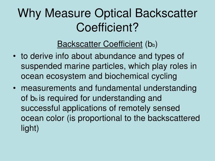
Why Measure Optical Backscatter Coefficient?. Backscatter Coefficient (b b ) to derive info about abundance and types of suspended marine particles, which play roles in ocean ecosystem and biochemical cycling

E N D
Why Measure Optical Backscatter Coefficient? Backscatter Coefficient (bb) • to derive info about abundance and types of suspended marine particles, which play roles in ocean ecosystem and biochemical cycling • measurements and fundamental understanding of bb is required for understanding and successful applications of remotely sensed ocean color (is proportional to the backscattered light)
What is optical backscattering? • bb is defined by all the photons incident on a particle that are redirected in the backward direction • bb + bf = b (total scattering coefficient)
Backscatter Coefficient • For a given distance of water, r, the fraction of incident light beam that is lost to back scattering equals: exp (-bb r) • bb is the sum of backscatter from all constituents (i.e. water molecules, salts, dissolved materials, organic and inorganic particles and BUBBLES
What does bb depend on? • Concentration of particles • Composition (Index of refraction) • Particle size distribution • Shape of particles
Even with same total volume of particles per given volume of water bb can be very different • Different optical properties respond differently to particle characteristics (size & composition) n > 1.15 is inorganic matter Volume Specific n = bb size = bb • Volume specific backscattering coef. (mie theory) of non-absorbing particles is shown to be strong function of size and composition of particles Plots derived from mie theory
Differences between the backscattering (bb) and scattering (b) dependence on particle composition and size suggests that they can be used together to obtain info about particle characteristics Therefore bb / b can be used to obtain information about the primary contributors to scattering in water Using backscattering and scattering
How do we measure Backscatter Coefficient? • Measured at limited number of angles between 100 and 155 degrees • Commercially available instruments measure one to three of these angles • Calibration • Done by using spherical beads with known optical properties • Or by measuring scattering properties of plate of known reflectivity
Single angle backscattering sensor -The more exact the detector is at receiving from a single angle the better the measurement
Again, the Link • Backscattering coefficient serves as proxy for amount of suspended matter in water • Reflectance of ocean surface (ocean color) is proportional to backscattering coefficient
Less stratified period Stratified periods had distinct 3-5 m cold layers, with warmer surface layer High absorption (676nm) due to high chl a conc. Yet shows almost no sign of backscatter Sediment re-suspension For water molecules and particles very small compared to wavelength of light, the backscattering ratio is ½ Phytoplankton dominated waters have backscatter ratio of ½ a percent And inorganic sedimenthave backscattering ratios of a few percent Backscattering ratio is highest yet still very small
Issues to consider • Paucity of measurements of marine particles • Particles deviate from spheres and homogeneity • Limited sub-micrometer particle size distribution, which is needed to understand scattering sources and variability
Ch. 5In Situ Measurement of the Inherent Optical Properties (IOPs) and Potential for Harmful Algal Bloom Detection and Coastal Ecosystem Observations
IOP concepts and measurement theory • The IOPs are defined as those properties describing the probability of photon removal and photon redirection i.e. absorption, scattering and beam attenuation coefficients and volume scattering function (VSF; β) • c = a+b • a, b, and c are linear sums of their constituent parts
Figure 5.3. Diagram of the scattering angles, q, where the bold arrow at left signifies the incident beam, forward scattering is indicated by the solid arrow and angle qf, and backscattering by the dashed arrow and angle qb. Forward scattering occurs in the forward white hemisphere (q = 0 to p/2) while backscattering occurs in the backward shaded hemisphere (q = p/2 to p) and azimuthal symmetry is assumed. In a bulk sense, the symmetry assumption holds in the ocean because, although particles are neither spherical nor homogeneous, they are randomly oriented. VSF • The VSF describes the angular distribution of scattering relative to the direction of light propagation, θ, and azimuthal angle φ axial symmetric
Φo is the incident radiant flux ΦA, ΦB, and ΦT are the absorbed, scattered and transmitted radiant flux The absorptance, scatterance and transmittance absorption coefficient, a, is the absorptance per unit distance in the layer, Δr 5.2 IOP concepts and measurement theory
Integrate previous equation for a. This equation yields two important pieces of information, first that the absorbed radiant flux is a function of path length (the longer the path, the greater the loss of radiant flux to absorption) and second, that the radiant flux decays exponentially along that path 5.2 IOP concepts and measurement theory
5.2 IOP concepts and measurement theory Similar arguments hold for the scattering and beam attenuation coefficients as well as the VSF:
5.2 IOP concepts and measurement theory Throughout this manuscript we will assume a simple theoretical size distribution of idealized particles given by a power-law (sometimes referred to as hyperbolic or Junge-like) function
5.3 IOP measurement reality it is impossible to measure the IOPs as defined theoretically in the previous section due to errors incurred by physical and electronic limitations in instrumentation However IOPs can be estimated with significant accuracy with proper instrument characterization, and corrections for the limitations
5.3 IOP measurement reality • Beam c – attenuation • Absorption • Scattering (VSF, backscattering)
Beam c • detector should have an infinitely small acceptance angle to exclude far-forward scattered light • there are physical limitations to the detector acceptance angle which introduces error which depends on VSF (below)
Figure 5.6. Conceptual diagram of the radiant flux in a beam transmissometer in which incident flux, Φo is multiply scattered (red arrows, ΦB) or transmitted (white arrows, ΦT) into the detector. In this case the geometric path length, r, is smaller than the optical path length for some photons, described by the sum of the red arrows. Beam c • Ideally the optical path length (i.e. the distance that photons travel between source and detector) is equal to the geometric path length of the sample compartment • Problems with multi-scattering
Figure 5.7. Conceptual diagram of the radiant flux in a reflecting tube absorption meter in which incident flux is absorbed, transmitted, scattered into the detector, reflected off the side walls into the detector, scattered out of the cuvette, or multiply scattered. Absorption • AC-9 only commerical in situ meter • Absorption measured with the WET Labs ac-9 is similar to a beam attenuation measurement, with the exception that the configuration is optimized to collect scattered light • Scattered light not collected leads to overestimation of absorption
Scattering • Direct scattering coefficients difficult to measure b/c can’t quantify absorbed flux • Therefore scattering coefficients gotten from b=c-a. • A distinction between sensors that measure scattering coefficient or VSF at a specific angle and those that measure scattering to determine particle concentration (i.e. turbidity or nephelometers).
Figure 5.8. Conceptual diagram of a single angle backscattering sensor. The incident irradiance, Φo, is a divergent beam with a known solid angle (bold arrow), the detector, likewise has a known detection solid angle. The detected scattered flux, ΦB (bold red arrow), occurs about the central backscattering angle, θ, within a volume (cyan) defined by the intersection of the incident and detected solid angles. The geometric path length is defined by the sum of the geometric lengths of the bold arrows. Simplified from Maffione and Dana (1997). Scattering - VSF No commercail sensor availible for complete VSF measurements. Although in the 70’s select measurements were made with the General Angle Scattering Meter (GASM) at 1 degree resolution.
Scattering - backscatter • The backscattering coefficient is currently determined from one or more measurements of the VSF at θ > 90º. Can measure backscatter at 3 angles to get a polynomial fit. Then integrate to get bb.
Calibration • Unavoidable sources of instrument variations with time include changes in lamp output magnitude and spectral dependence, detector degradation and response, and filter degradation and response • Avoidable sources of instrument variation include dirty instrumentation, incorrect configurations, and inappropriate blanks • Factory calibration recommended but not always possible
Environmental Sensitivity • Electronic instrumentation often exhibits sensitivity to ambient temperature • Optical instruments that depend upon precise alignment may exhibit sensitivity to ambient pressure • dependence of the reference material IOPs on temperature must be quantified in addition to the instrument response to temperature (i.e. the dependence of the pure water running through the sample compartment or the sample volume and the dependence of the instrument in water of a temperature different from room temperature)
Figure 5.14. A. Volume scattering functions for a range of particle concentrations (1 to 50 arbitrary units) for particles obeying a Junge distribution with slope of 4 and a refractive index of 1.05 + i 0.001. B. Modeled values for beam attenuation coefficient coefficients for the samples in part A that would result from measurements made with a LISST and an ac‑9 versus the theoretical beam attenuation coefficients, given their detection angle responses. IOP Measurement Sensitivity to Particle Concentration
Figure 5.15. A. Volume scattering functions for particles with a range of real refractive index, obeying a Junge distribution with a slope of 4 and with an imaginary refractive index of 0.001. Curves have been normalized to total particle volume to remove the effects of biomass. Inset shows the first 2o of resolution on a linear scale. B. The beam attenuation coefficients for the samples in part A that would result from measurements made with the two instruments versus the theoretical values, as in Figure 5.14. IOP Measurement Sensitivity to Composition (real refractive index)
Forward Volume Scattering Function Meter Sensitivity • Use the forward VSF to estimate the shape of the particle size distribution for particles without accounting for their refractive index (composition)
Backward volume scattering meter sensitivity • To first order, the backscattering increases as the concentration of particles increases • To second order, backscattering increases as the real refractive index increases and as the imaginary refractive index decreases (i.e. weakly absorbing particles are more efficient backscatters compared to strongly absorbing particles because photons that enter particles are more likely to be absorbed and thus are not available to be backscattered)
Backward volume scattering meter sensitivity • Algal cells, and other strongly absorbing particles, exhibit the lowest backscattering ratios (~0.5%) due to their large water content • weakly-absorbing organic and detrital particles have higher ratios (near 1%) • inorganic particles have the highest ratios (~2%) • But particle absorption can cause uncertainty
Sensitivity of side or wide angle scattering meters (turbidometers, nephelometers) • Side angles or wide angle scattering have been used historically to quantify the suspended particle mass • Dependence of the magnitude of the side scattering on, not only particle concentration, but particle composition (real refractive index) and size distribution
Figure 5.21. An example of the characterization of the WET Labs LSS sensor using dilutions of inorganic clay particles of known size distribution. A. Size distribution of six clay-particle suspensions, determined by Coulter Counter. Vertical lines indicate modal diameter for each suspension. B. LSS response (NTU) to dilutions of the six suspensions, each represented by data points along a line color coded to the size distribution as in part A. The slope of the line is the concentration-specific backscattering coefficient, Kbs (NTU.(mg.l-1)-1). C. Dependence of the concentration-specific backscattering coefficient, Kbs, on the mean particle diameter for each suspension, data point color coded as in parts A and B. Modified from Baker et al. (2001). This demonstrates that the LSS is most sensitive to particles in the size range 1 mm and less sensitive to both larger and smaller particles.
What are the Particles Responsible for Scattering in the Ocean? Figure 5.22. Particle volume-specific instrument response as a function of particle diameter for a A. beam transmissometer, B. wide-angle scattering sensor, C. single-angle backscattering sensor, as a function of particle refractive indices (ranging 1.05 to 1.24). As particle refractive index increases, all scattering properties increase. Beam c is most sensitive to highly refractive (i.e. mineralic) particles in the range of 1 µm. For less refractive particles (i.e. phytoplankton), beam c is most sensitive to particles of diameter 5 µm. Wide angle side scattering is most sensitive to particles in the size range 0.5 µm, regardless of refractive index although the response increases with refractive index. Backscattering is most sensitive to small particles of order 0.2 µm although the relationship is complicated and particles up to 5 µm are effective backscatterers.
Figure 5.23. Example of the contribution of particles within discrete size ranges to the total particle backscattering for natural waters. A. The cumulative backscattering as a function of particle diameter for discrete size intervals. The total particle backscattering coefficient is indicated by the dotted line (~ 0.105 m-1) and error bars indicate 1 standard deviation of >300 realizations. B. The percent contribution to total backscattering by each size interval. A whole water sample collected from the Damariscotta River Estuary was size fractioned (ranges indicated by bars) and the backscattering of each fraction was measured with a WET Labs ECOvsf sensor (440 nm). For this particular sample, which is consistent with other collected during a 24-hour time series experiment, the particles in the 3-10 µm size range dominated the backscattering coefficient. This results in part from their particle-specific backscattering efficiency (which is modeled in Figure 5.22) and their in situ concentration relative to particles in the other size intervals. In terms of phytoplankton, only the very small picoplankton would be significant contributors to the particle backscattering. Larger phytoplankton are inefficient backscatterers because of their larger size and because of their strong absorption (imaginary refractive indices).
What is the IOP measurement response to algal blooms? • Phytoplankton exhibit a great impact on IOPs because of their spectrally-varying imaginary refractive index, n' • Results in variations in magnitude and spectral shape of absorption and scattering spectra • Spectra gets more complicated as the proportion of phyto. plankton cells increases relative to non-algal particles • spectral shape changes as pigment ratios vary in response to species composition • spectral shape of the phytoplankton absorption varies in response to algal cell size and nutrient and light conditions due to packaging of the pigment within the cell
HAB IOP examples Figure 5.25. Measured inherent optical properties of two algal blooms, Prorocentrum micans (red) in the Gulf of Maine and Aureococcus anophagefferens (brown) in Long Island Sound. The algae were of sufficient concentrations to turn the water red and brown, respectively. The a and c coefficients were measured with an ac-9, and used to derive b. The measured IOPs and particle size distributions were used to estimate indices of refraction at the ac-9 wavelengths and backscattering was determined using Mie modeling. Note that the P. micans values in parts B-D have been multiplied by 5 for ease of resolving spectral shapes. Flattening of blue peak in absoption The spectral slope of the beam c was flat, consistent with dominance by large particles The backscattering ratio was ~ 0.2% consistent with large, strongly absorbing algal cells
Figure 5.26. Examples of water discoloration during the monospecific HABs in Figure 5.25. A and B. View of coastal waters near Bigelow Laboratory for Ocean Sciences, West Boothbay Harbor Maine, in October 1999, prior to (A) and during (B) the P. micans bloom. The water is characteristically green due to high CDM absorption and red during the bloom due to the enhanced blue-green absorption and red backscattering of the P. micans cells. (Photos courtesy of M. Keller.) C. Brown water associated with the Aureococcus anophagefferens bloom in Quantuck Bay, Long Island, New York in June 2000. Photo courtesy of S. Etheridge.
IOP observations contribute important info about HABS • These include the detection of changes • in algal a to total a • in spectral slope of beam attenuation, indicating bulk particle changes • in bulk scattering ratio, indicating changing dominant algal species • In near forward VSF, indicating change in bulk size distribution
Estimation of slope of particle size distribution derived from spectral slope of beam c indicate that QB Bay was dominated by smaller particles (Brown Tide – A. Anophagefferens) Large variations in estimated particle size slope observed in WNB bay (no brown tide) Long Island Sound
Off the Coast of Florida Spectral IOPs provide indicators of target species among background of phytoplankton community • Depend on the capability for in situ hyperspectral absorption and algorithms to identify specific pigments composition (K. Brevis)
The Gulf of Maine Two separate de-stratification events Temporal Variations in Ecosystem inferred by IOPs De-convolution of spectral absorption coefficients yielded 2 different spectral shapes for phytoplankton absorption Complete de-stratification Period of low backscatter ratio, high algal concentration Second bloom occurs when very mixed waters
The Future • Further miniaturization • Filter Cartridges • Isolate target species • Acidification • Dissolve carbonate cell walls • Pressurization • Burst gas vacuoles (cyanobacteria)
Chuck Norris Completely Irrelevant Picture of Perfect Rincon The End