Download

1 / 62
620 likes | 655 Views
Dive into software metrics concepts, including direct and indirect measures, product vs. process metrics, size-oriented metrics, complexity metrics like Halstead’s and McCabe’s, and the importance of interpreting data for software quality improvement.

E N D
Software Metrics Disclaimer There’s a plethora of testing tools and static analyzers that compute metrics. We will not be focusing here on tools but rather on concepts.
Definitions • Measure - quantitative indication of extent, amount, dimension, capacity, or size of some attribute of a product or process. • E.g., Number of errors • Metric - quantitative measure of degree to which a system, component or process possesses a given(quality?) attribute. “A handle or guess about a given(quality?) attribute.” • E.g., Number of errors found per person hours JP’s take: metrics need interpretation
Motivation for Metrics • Estimate the cost & schedule of future projects • Evaluate the productivity impacts of new tools and techniques • Establish productivity trends over time • Improve software quality • Forecast future staffing needs • Anticipate and reduce future maintenance needs
Example Metrics • Defect rates • (where a defect is something less serious than an error wrtreqs) • Error rates: Errors should be categorized by origin, type, cost • It is a luxury to invest in root cause analysis • Measured wrt: • individual • Module/class/procedure
Product vs. Process • Process Metrics • Insights of process paradigm, software engineering tasks, work product, or milestones • Lead to long term process improvement • Product Metrics • Assess the state of the project • Track potential risks • Uncover problem areas • Adjust workflow or tasks • Evaluate teams ability to control quality
Types of Measures • Direct Measures (internal attributes) • Cost ($$), effort (in man/days), LOC (lines of code), response speed, memory footprint • white box viewpoint • Indirect Measures (external attributes) • Functionality, complexity, efficiency, reliability, maintainability (more on this later in the course) • Black box viewpoint • Both pertain to quality?
Size-Oriented Metrics Size of the software produced: • LOC - Lines Of Code • KLOC - 1000 Lines Of Code • SLOC –Statement Lines of Code (ignore whitespace) • Popular because easy to compute • Typical Measures: • Errors/KLOC, Defects/KLOC, Cost/LOC, Documentation Pages/KLOC
Complexity Metrics • LOC - a ‘rough’ function of complexity • Halstead’s Software Science • (entropy measures, i.e., measures towards (quality?) equilibrium…) • n1 - number of distinct operators • n2 - number of distinct operands • N1 - total number of operators • N2 - total number of operands
Example if (k < 2) { if (k > 3) x = x*k; } • Distinct operators: if ( ) { } > < = * ; • Distinct operands: k 2 3 x • n1 = 10 • n2 = 4 • N1 = 13 • N2 = 7
Halstead’s Metrics • Amenable to experimental verification [1970s] • Program length: N = N1 + N2 (in ex: 20) • Program vocabulary: n = n1 + n2 (in ex: 14) • Volume V = N * log2n(in ex: 76.14) • Difficulty D = (n1/2) + (N2/n2) (in ex: 6.75) • Effort E = D x V (in ex:514) • Time to program T = (E / 18) seconds (in ex: 29 s) • Number of delivered bugs B = V / 3000 (in ex: 0.025) • Welcome to the science of metrics, for which interpretation is often an art… For example, D and E are taken to pertain to understandability…
McCabe’s Complexity Measures • McCabe’s metrics are based on a control flow representation of the program. • Acontrol flow graph is used to depict control flow. • Nodes represent processing tasks (one or more code statements) • Edges represent control flow between nodes
Flow Graph Notation While Sequence If-then-else Until
Cyclomatic Complexity • Defined as the set of independent paths through the control flow graph • V(G) = E – N + 2 • E is the number of flow graph edges • N is the number of nodes • V(G) = P + 1 • P is the number of predicate nodes
Example i = 0; while (i<n-1) do j = i + 1; while (j<n) do if A[i]<A[j] then swap(A[i], A[j]); end do; i=i+1; end do;
Flow Graph 1 2 3 7 4 5 6
Computing V(G) • V(G) = 9 – 7 + 2 = 4 • V(G) = 3 + 1 = 4 • Basic paths are: • 1, 7 • 1, 2, 6, 1, 7 • 1, 2, 3, 4, 5, 2, 6, 1, 7 • 1, 2, 3, 5, 2, 6, 1, 7
Meaning of V(G) • Complexity increases with the number of decision paths and loops • V(G) is a quantitative measure of the testing difficulty and, ultimately, an indication of reliability • Experimental data shows value of V(G) should be no more then 10: testing is very difficult above this value
McClure’s Complexity Metric • Complexity = C + V • C is the number of comparisons in a module • V is the number of control variables referenced in the module (from ifs and loops) • Targets decisional complexity • Somewhat pertains to path sensitization • Similar to McCabe’s but with regard to control variables. • Can this be correlated to software quality?
A Comment McCall’s quality factors were proposed in the early 1970s. They appear to be as valid today as they were at that time. It’s likely that software built to conform to these factors will exhibit high quality well into the 21st century, even if there are dramatic changes in technology.
product operation revision transition reliability efficiency usability maintainability testability portability reusability Quality Model(is ISO 9126 relevant to this?) Metrics
High Level Design Metrics • Structural Complexity • Data Complexity • System Complexity • Structural Complexity S(i) of a module i. • S(i) = fout2(i) • Fan out is the number of modules immediately subordinate (directly invoked).
Design Metrics • Data Complexity D(i) • D(i) = v(i)/[fout(i)+1] • v(i) is the number of inputs and outputs passed to and from i • System Complexity C(i) • C(i) = S(i) + D(i) • As eachC(i) increases the overall complexity of the architecture increases
System Complexity Metric • Another metric: • length(i) * [fin(i) + fout(i)]2 • Length is LOC • Fan in is the number of modules that invokei • The real question: what are ‘good’ numbers for each of these metrics?
Coupling for a module • Data and control flow: (a key distinction) • di input data parameters • ci input control parameters • do output data parameters • co output control parameters • Global • gd global variables for data • gc global variables for control • Environmental • w fan in • r fan out
Metrics for Coupling • Mc = k/m, k=1 • m = di + aci + do + bco + gd + cgc + w + r • Key point: a, b, c, k can be adjusted based on actual data… but how is this done? • This computation can be so subjective that most will rely on simpler (if not simplistic) metrics…
Component Level Metrics • Cohesion (internal interaction) – pertains to data members • Coupling (external interaction) - a function of input and output parameters, global variables, and modules called • Complexity of program flow - hundreds have been proposed (e.g., cyclomatic complexity) • Cohesion – difficult to measure • Bieman ’94, TSE 20(8)
Using Metrics • The Process • Select appropriate (??) metrics for problem • Use metrics on problem • Assess and generate feedback • Steps: • Formulation • Collection • Analysis • Interpretation • Feedback
Metrics for the Object Oriented • Chidamber & Kemerer ’94 TSE 20(6) • Metrics specifically designed to address object-oriented software • Class-oriented metrics: • No need for procedure level metrics • Cluster level metrics is simply too complex • Simple direct measures
Chidamber and Kemerer Metrics • Weighted methods per class (MWC) • Depth of inheritance tree (DIT) • Number of children (NOC) • Coupling between object classes (CBO) • Response for class (RFC) • Lack of cohesion metric (LCOM)
ci is the complexity of each method Mi of the class Often, only public methods are considered Complexity may be the McCabe complexity of the method Smaller values are better Perhaps the average complexity per method is a better metric Weighted methods per class (WMC)
Weighted Methods per Class • Viewpoints from Chidamberand Kemerer:-The number of methods and complexity of methods is an indicator of how much time and effort is required to develop and maintain the object-The larger the number of methods in an object, the greater the potential impact on the children-Objects with large number of methods are likely to be more application specific, limiting possible reuse
Depth of inheritance tree (DIT) • For the system under examination, consider the hierarchy of classes • DIT is the length of the maximum path from the node to the root of the tree • Relates to the scope of the properties • How many ancestor classes can potentially affect a class • Smaller values are better
Number of children (NOC) • For any class in the inheritance tree, NOC is the number of immediate children of the class • The number of direct subclasses • How would you interpret this number? • A moderate (??) value indicates scope for reuse and high values may indicate an inappropriate abstraction in the design
Number of Children • Viewpoints: • As NOC grows, reuse increases - but the abstraction may be diluted • Depth is generally better than breadth in class hierarchy, since it promotes reuse of methods through inheritance • Really?? Open-closed principle? Does this not contradict heuristic for DIT? • Classes higher up in the hierarchy should have more sub-classes then those lower down • NOC gives an idea of the potential influence a class has on the design: classes with large number of children may require more testing
Coupling between Classes • CBO is the number of collaborations between two classes (fan-out of a class C) • the number of other classes that are referenced in the class C (where a reference to another class, A, is a reference to a method or a data member of class A) • Viewpoints: • High fan-outs denote class coupling to other classes/objects and thus are undesirable. High fan-ins denote good designs and a high level of reuse • Not possible to maintain high fan-in and low fan outs across the entire system • Excessive coupling indicates weakness of class encapsulation and may inhibit reuse • High coupling also indicates that more faults may be introduced due to inter-class activities
Response for class (RFC) • Mci:# of methods called in response to a message that invokes method Mi • Fully nested set of calls • Smaller numbers are better • Larger numbers indicate increased complexity and debugging difficulties If a large number of methods can be invoked in response to a message, the testing and debugging of the class becomes more complicated
Lack of cohesion metric (LCOM) • Number of methods in a class that reference a specific instance variable • A measure of the “tightness” of the code • If a method references many instance variables, then it is more complex and less cohesive • The larger the number of similar methods in a class the more cohesive the class is • “Cohesion of methods within a class is desirable, since it promotes encapsulation” (??)
Lack of Cohesion in Methods • LCOM – poorly described in Pressman • Class Ck with n methods M1,…Mn • Ij is the set of instance variables used by Mj
LCOM • There are n such sets I1 ,…, In • P = {(Ii, Ij) | (Ii Ij ) = } //no common inst. var. • Q = {(Ii, Ij) | (Ii Ij ) } • If all n sets Ii are then P = • LCOM = |P| - |Q|, if |P| > |Q| • LCOM = 0 otherwise
Example LCOM • Take class C with M1, M2, M3 • I1 = {a, b, c, d, e} • I2 = {a, b, e} • I3 = {x, y, z} • P = {(I1, I3), (I2, I3)} //those do not intersect • Q = {(I1, I2)} //those that do • Thus LCOM = 1
Explanation • LCOM is the number of empty intersections minus the number of non-empty intersections • This is a notion of degree of similarity of methods • If two methods use common instance variables then they are (??) similar • LCOM of zero is not maximally cohesive • |P| = |Q| or |P| < |Q|
Class Size • CS • Total number of operations (inherited, private, public) • Number of attributes (inherited, private, public) • May be an indication of too much responsibility for a class
Number of Operations Overridden • NOO • A large number for NOO indicates possible problems with the design • Poor abstraction in inheritance hierarchy
Number of Operations Added • NOA • The number of operations added by a subclass • As operations are added the subclass ‘moves away’ from the parent class • As depth increases NOA should decrease
Method Inheritance Factor MIF = . • Mi(Ci) is the number of methods inherited and not overridden in Ci • Ma(Ci) is the number of methods that can be invoked with Ci(see next slide) • Md(Ci) is the number of methods declared in Ci(see next slide)
MIF • Ma(Ci) = Md(Ci) + Mi(Ci) • Meaning: All that can be invoked = (new or overloaded) + things inherited • MIF is [0,1] • MIF near 1 means little specialization • MIF near 0 means large change
Coupling Factor CF= . • is_client(x,y) = 1 iff a relationship exists between the client class and the server class. 0 otherwise • (TC2-TC) is the total number of relationships possible (where TC is the # of classes) • Entails relationships are not bidirectional • Formula calculates xproduct - diagonal • CF is [0,1] with 1 meaning high coupling