Download
1 / 64
640 likes | 791 Views
Embedded Systems in Silicon TD5102 Compilers with emphasis on ILP compilation. Henk Corporaal http://www.ics.ele.tue.nl/~heco/courses/EmbSystems Technical University Eindhoven DTI / NUS Singapore 2005/2006. Compiling for ILP Architectures. Overview: Motivation and Goals

E N D
Embedded Systems in SiliconTD5102Compilerswith emphasis on ILP compilation Henk Corporaal http://www.ics.ele.tue.nl/~heco/courses/EmbSystems Technical University Eindhoven DTI / NUS Singapore 2005/2006
Compiling for ILP Architectures Overview: • Motivation and Goals • Measuring and exploiting available parallelism • Compiler basics • Scheduling for ILP architectures • Summary and Conclusions
Motivation • Performance requirements increase • Applications may contain much instruction level parallelism • Processors offer lots of hardware concurrency Problem to be solved: • how to exploit this concurrency automatically?
Goals of code generation • High speedup • Exploit all the hardware concurrency • Extract all application parallelism • obey true dependencies only • resolve false dependencies by renaming • No code rewriting: automatic parallelization • However: application tuning may be required • Limit code expansion
Overview • Motivation and Goals • Measuring and exploiting available parallelism • Compiler basics • Scheduling for ILP architectures • Summary and Conclusions
Measuring and exploiting available parallelism • How to measure parallelism within applications? • Using existing compiler • Using trace analysis • Track all the real data dependencies (RaWs) of instructions from issue window • register dependence • memory dependence • Check for correct branch prediction • if prediction correct continue • if wrong, flush schedule and start in next cycle
Execution trace set r1,0 set r2,3 set r3,&A st r1,0(r3) add r1,r1,1 add r3,r3,4 brne r1,r2,Loop st r1,0(r3) add r1,r1,1 add r3,r3,4 brne r1,r2,Loop st r1,0(r3) add r1,r1,1 add r3,r3,4 brne r1,r2,Loop add r1,r5,3 Trace analysis Compiled code set r1,0 set r2,3 set r3,&A Loop: st r1,0(r3) add r1,r1,1 add r3,r3,4 brne r1,r2,Loop add r1,r5,3 Program For i := 0..2 A[i] := i; S := X+3; How parallel can this code be executed?
Trace analysis Parallel Trace set r1,0 set r2,3 set r3,&A st r1,0(r3) add r1,r1,1 add r3,r3,4 st r1,0(r3) add r1,r1,1 add r3,r3,4 brne r1,r2,Loop st r1,0(r3) add r1,r1,1 add r3,r3,4 brne r1,r2,Loop brne r1,r2,Loop add r1,r5,3 Max ILP = Speedup = Lparallel / Lserial = 16 / 6 = 2.7
Ideal Processor Assumptions for ideal/perfect processor: 1. Register renaming– infinite number of virtual registers => all register WAW & WAR hazards avoided 2. Branch and Jump prediction– Perfect => all program instructions available for execution 3. Memory-address alias analysis– addresses are known. A store can be moved before a load provided addresses not equal Also: • unlimited number of instructions issued/cycle (unlimited resources), and • unlimited instruction window • perfect caches • 1 cycle latency for all instructions (FP *,/) Programs were compiled using MIPS compiler with maximum optimization level
Upper Limit to ILP: Ideal Processor Integer: 18 - 60 FP: 75 - 150 IPC
Different effects reduce the exploitable parallelism • Reducing window size • i.e., the number of instructions to choose from • Non-perfect branch prediction • perfect (oracle model) • dynamic predictor (e.g. 2 bit prediction table with finite number of entries) • static prediction (using profiling) • no prediction • Restricted number of registers for renaming • typical superscalars have O(100) registers • Restricted number of other resources, like FUs
Different effects reduce the exploitable parallelism • Non-perfect alias analysis (memory disambiguation)Models to use: • perfect • inspection: no dependence in following cases: r1 := 0(r9) r1 := 0(fp) 4(r9) := r2 0(gp) := r2 A more advanced analysis may disambiguate most stack and global references, but not the heap references • none • Important: • good branch prediction, 128 registers for renaming, alias analysis on stack and global accesses, and for FloatingPt a large window size
Summary • Amount of parallelism is limited • higher in Multi-Media • higher in kernels • Trace analysis detects all types of parallelism • task, data and operation types • Detected parallelism depends on • quality of compiler • hardware • source-code transformations
Overview • Motivation and Goals • Measuring and exploiting available parallelism • Compiler basics • Scheduling for ILP architectures • Source level transformations • Compilation frameworks • Summary and Conclusions
Compiler basics • Overview • Compiler trajectory / structure / passes • Abstract Syntax Tree (AST) • Control Flow Graph (CFG) • Data Dependence Graph (DDG) • Basic optimizations • Register allocation • Code selection
Compiler basics: trajectory Source program Preprocessor Compiler Error messages Assembler Library code Loader/Linker Object program
Compiler basics:structure / passes Source code Lexical analyzer token generation check syntax check semantic parse tree generation Parsing Intermediate code data flow analysis local optimizations global optimizations Code optimization code selection peephole optimizations Code generation making interference graph graph coloring spill code insertion caller / callee save and restore code Register allocation Sequential code Scheduling and allocation exploiting ILP Object code
:= id + id * id 60 Compiler basics: structure Simple compilation example position := initial + rate * 60 Lexical analyzer temp1 := intoreal(60) temp2 := id3 * temp1 temp3 := id2 + temp2 id1 := temp3 id := id + id * 60 Syntax analyzer Code optimizer temp1 := id3 * 60.0 id1 := id2 + temp1 Code generator movf id3, r2 mulf #60, r2, r2 movf id2, r1 addf r2, r1 movf r1, id1 Intermediate code generator
FORTRAN C FORTRAN to C pre-processing C front-end FORTRAN specific transformations converting non-standard structures to SUIF constant propagation forward propagation high-SUIF to low-SUIF induction variable identification constant propagation scalar privatization analysis strength reduction reduction analysis dead-code elimination locality optimization and parallelism analysis register allocation parallel code generation assembly code generation SUIF to text SUIF to postscript SUIF to C postscript SUIF text assembly code C Compiler basics: structure - SUIF-1 toolkit example
Compiler basics:Abstract Syntax Tree (AST) C input code: Parse tree: ‘infinite’ nesting: if (a > b) { r = a % b; } else { r = b % a; } Stat IF Cmp > Var a Var b Statlist Stat Expr Assign Var r Binop % Var a Var b Statlist Stat Expr Assign Var r Binop % Var b Var a
Compiler basics:Control flow graph (CFG) C input code: if (a > b) { r = a % b; } else { r = b % a; } 1 sub t1, a, b bgz t1, 2, 3 CFG: 2 rem r, a, b goto 4 3 rem r, b, a goto 4 4 ………….. ………….. Program, is collection of Functions, each function is collection of Basic Blocks, each BB contains set of Instructions, each instruction consists of several Transports,..
Data Dependence Graph (DDG) a := b + 15; c := 3.14 * d; e := c / f; Translation to DDG &d ld 3.14 &f &b ld ld * 15 &c + / st &a &e st st
Compiler basics: Basic optimizations • Machine independent optimizations • Machine dependent optimizations (details are in any good compiler book)
Machine independent optimizations • Common subexpression elimination • Constant folding • Copy propagation • Dead-code elimination • Induction variable elimination • Strength reduction • Algebraic identities • Commutative expressions • Associativity: Tree height reduction • Note: not always allowed(due to limited precision)
Machine dependent optimization example What’s the optimal implementation of a*34 ? • Use multiplier: mul Tb,Ta,34 • Pro: No thinking required • Con: May take many cycles • Alternative: SHL Tc, Ta, 1 ADD Tb, Tc, Tzero SHL Tc, Tc, 4 ADD Tb, Tb, Tc • Pros: May take fewer cycles • Cons: • Uses more registers • Additional instructions ( I-cache load / code size)
Compiler basics: Register allocation • Register Organization Conventions needed for parameter passing and register usage across function calls; a MIPS example: r31 Callee saved registers r21 Caller saved registers r20 Temporaries r11 r10 Argument and result transfer r1 Hard-wired 0 r0
Register allocation using graph coloring Given a set of registers, what is the most efficient mapping of registers to program variables in terms of execution time of the program? • A variable is defined at a point in program when a value is assigned to it. • A variable is used at a point in a program when its value is referenced in an expression. • The live range of a variable is the execution range between definitions and uses of a variable.
Program: • a := • c := • b := • := b • d := • := a • := c • := d a b c d Register allocation using graph coloring Example: Live Ranges
a b c d Register allocation using graph coloring Inference Graph a • Coloring: • a = red • b = green • c = blue • d = green b c d Graph needs 3 colors (chromatic nr =3) => program needs 3 registers
Program: • a := • c := • store c • b := • := b • d := • := a • load c • := c • := d Live Ranges a b c d Register allocation using graph coloring Spill/ Reload code Spill/ Reload code is needed when there are not enough colors (registers) to color the interference graph Example: Only two registers available !!
Compiler basics: Code selection • CISC era • Code size important • Determine shortest sequence of code • Many options may exist • Pattern matching Example M68020: D1 := D1 + M[ M[10+A1] + 16*D2 + 20 ] ADD ([10,A1], D2*16, 20), D1 • RISC era • Performance important • Only few possible code sequences • New implementations of old architectures optimize RISC part of instruction set only; for e.g. i486 / Pentium / M68020
Overview • Motivation and Goals • Measuring and exploiting available parallelism • Compiler basics • Scheduling for ILP architectures • Source level transformations • Compilation frameworks • Summary and Conclusions
What is scheduling? • Time allocation: • Assigning instructions or operations to time slots • Preserve dependences: • Register dependences • Memory dependences • Optimize code with respect to performance/ code size/ power consumption/ .. • Space allocation • satisfy resource constraints: • Bind operations to FUs • Bind variables to registers/ register files • Bind transports to buses
Why scheduling? Let’s look at the execution time: Texecution = Ncycles x Tcycle = Ninstructions x CPI x Tcycle Scheduling may reduce Texecution • Reduce CPI (cycles per instruction) • early scheduling of long latency operations • avoid pipeline stalls due to structural, data and control hazards • allow Nissue > 1 and therefore CPI < 1 • Reduce Ninstructions • compact many operations into each instruction (VLIW)
Unscheduled code: Lw R1,b Lw R2,c Add R3,R1,R2 interlock Sw a,R3 Lw R1,e Lw R2,f Sub R4,R1,R2 interlock Sw d,R4 Scheduled code: Lw R1,b Lw R2,c Lw R5,e extra reg. needed! Add R3,R1,R2 Lw R2,f Sw a,R3 Sub R4,R5,R2 Sw d,R4 Scheduling data hazardsRaW dependence Avoiding RaW stalls: Reordering of instructions by the compiler Example: avoiding one-cycle load interlock Code: a = b + c d = e - f
time IF ID OF EX Branch L IF ID OF EX WB Predict not taken IF ID OF EX WB IF ID OF EX WB IF ID OF EX WB L: Scheduling control hazards Branch requires 3 actions: • Compute new address • Determine condition • Perform the actual branch (if taken): PC := new address
Control hazards: what's the penalty? CPI = CPIideal + fbranch x Pbranch Pbranch = Ndelayslots x miss_rate • Superscalars tend to have large branch penalty Pbranch due to • many pipeline stages • multiple instructions (or operations) / cycle • Note: • the lower CPI the larger the effect of penalties
What can we do about control hazards and CPI penalty? • Keep penalty Pbranch low: • Early computation of new PC • Early determination of condition • Visible delay slots filled by compiler (MIPS) • Branch prediction • Reduce control dependencies (control height reduction) [Schlansker and Kathail, Micro’95] • Remove branches: if-conversion • Conditional instructions: CMOVE, cond skip next • Guarding all instructions: TriMedia
Scheduling: Conditional instructions After conversion: • Example: Cmove (supported by Alpha) If (A=0) S = T; assume: r1: A, r2: S, r3: T Object code: Bnez r1, L Mov r2, r3 L: . . . . Cmovz r2, r3, r1
Scheduling: Conditional instructions Conditional instructions are useful, however: • Squashed instructions still take execution time and execution resources • Consequence: long target blocks can not be if-converted • Condition has to be known early • Moving operations across multiple branches requires complicated predicates • Compatibility: change of ISA (instruction set architecture) Practice: • Current superscalars support a limited set of conditional instructions • CMOVE: alpha, MIPS, PowerPC, SPARC • HP PA: any RR instruction can conditionally squash next instruction Large VLIWs profit from making all instructions conditional • guarded execution: TriMedia, Intel/HP IA-64, TI C6x
Guarded execution SLT r1,r2,r3 BEQ r1,r0, else then: ADDI r2,r2,1 ..X.. j cont else: SUBI r2,r2,1 ..Y.. cont: MUL r4,r2 IF-conversion SLT b1,r2,r3 b1:ADDI r2,r2,1 !b1: SUBI r2,r2,1 b1:..X.. !b1: ..Y.. MUL r4,r2
Scheduling: Conditional instructions Full guard support If-conversion of conditional code Assume: • tbranch branch latency • pbranch branching probability • ttrue execution time of the TRUE branch • tfalse execution time of the FALSE branch Execution times of original and if-converted code for non-ILP architecture: toriginal_code = (1 +pbranch) xtbranch + pxttrue + (1 - pbranch) xtfalse tif_converted_code = ttrue + tfalse
Scheduling: Conditional instructions Speedup of if-converted code for non-ILP architectures Only interesting for short target blocks!
Scheduling: Conditional instructions Speedup of if-converted code for ILP architectures with sufficient resources tif_converted = max(ttrue, tfalse) Much larger area of interest !!
Scheduling: Conditional instructions • Full guard support for large ILP architectures has a number of advantages: • Removing unpredictable branches • Enlarging scheduling scope • Enabling software pipelining • Enhancing code motion when speculation is not allowed • Resource sharing; even when speculation is allowed guarding may be profitable
Scheduling: Overview Transforming a sequential program into a parallel program: read sequential program read machine description file for each procedure do perform function inlining for each procedure do transform an irreducible CFG into a reducible CFG perform control flow analysis perform loop unrolling perform data flow analysis perform memory reference disambiguation perform register allocation for each scheduling scope do perform instruction scheduling write parallel program
Scheduling: Int.Lin.Programming Integer linear programming scheduling method • Introduce: • Decision variables: xi,j = 1 if operation i is scheduled in cycle j • Constraints like: • Limited resources: where xtoperation of type t and Mtnumber of resources of type t • Data dependence constraints • Timing constraints • Problem: too many decision variables
List Scheduling • Make a dependence graph • Determine minimal length • Determine ASAP, ALAP, and slack of each operation • Place each operation in first cycle with sufficient resources Note: • Scheduling order sequential • Priority determined by used heuristic; e.g. slack
Basic Block Scheduling ASAP cycle B C ALAP cycle ADD A slack <1,1> A C SUB <2,2> ADD NEG LD <3,3> <1,3> <2,3> A B LD MUL ADD <4,4> <2,4> <1,4> z y X
min{alap(u) - delay(u,v) | (u,v) E } ifsucc(v) Lmax otherwise max{asap(u) + delay(u,v) | (u,v) E } ifpred(v) 0 otherwise asap(v) = alap(v) = ASAP and ALAP formulas slack(v) = alap(v) - asap(v)