Spring 2008 CSE 591 Compilers for Embedded Systems

Spring 2008 CSE 591Compilers for Embedded Systems Aviral Shrivastava Department of Computer Science and Engineering Arizona State University

Lecture 6: Scratch Pad Memories Management and Data Mapping Techniques

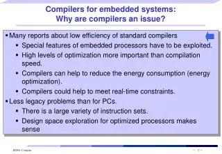
poor design techniques Energy Efficiency Operations/Watt[GOPS/W] Ambient Intelligence 10 DSP-ASIPs 1 Processors ASIC Reconfigurable Computing µPs 0.1 0.01 Technology 1.0µ 0.5µ 0.25µ 0.13µ 0.07µ Necessary to optimize; otherwise the price for flexibility cannot be paid! [H. de Man, Keynote, DATE‘02; T. Claasen, ISSCC99]

SPMs vs. Cache Energy consumption in tags, comparators and muxes is significant! [R. Banakar, S. Steinke, B.-S. Lee, 2001]

Advantages of Scratch Pads • Area advantage - For the same area, we can fit more memory of SPM than in cache (around 34%) • SPM consists of just a memory array & address decoding circuitry • Less energy consumption per access • Absence of tag memory and comparators • Performance comparable with cache • Predictable WCET – required for RTES

Systems with SPM • Most of the ARM architectures have an on-chip SPM termed as Tightly-coupled memory (TCM) • GPUs such as Nvidia’s 8800 have a 16KB SPM • Its typical for a DSP to have scratch pad RAM • Embedded processors like Motorola Mcore, TI TMS370C • Commercial network processors – Intel IXP • Cell Broadband Engine

Challenges in using SPMs • In SPMs, application developer, or compiler has explicitly move data between memories • Data mapping is transparent in cache based architectures • Binary compatible? • Do advantages translate to a different machine?

Data Allocation on SPM • Data Classification • Global data • Stack data • Heap data • Application Code • Mapping classification • Static – Mapping of data decided at compile time and the mapping persists throughout the execution • Dynamic – Mapping of data decided at compile time but the mapping changes throughout execution • Analysis Classification • Profile based analysis • Compile-time analysis • Goal Classification • To minimize off-chip memory access • To reduce energy consumption • To achieve better performance

Global Data • Panda et al., “Efficient Utilization of Scratch-Pad Memory in Embedded Processor Applications” • Map all scalars to SPM • Very small in size • Estimate conflicts in array • IAC(u): Interference Access Count: No. of accesses to other arrays during lifetime of u • VAC(u): Variable Access Count: Number of accesses to elements of u • IF(u) = ILT(u)*VAC(u) • Loop Conflict Graph • Nodes are arrays • Edge weight of (u -> v) is the number of accesses to u and v in the loop • More conflict  SPM • Either whole array goes to SPM or not

ILP for Global Variables • Memory units: m_i • Power per access of each memory: p_m_i • Number of times each variable is accessed: n_j • Compute where each variable should be placed to minimize the power consumption • Compiler decides where to place the global variables

ILP for Code+GVs • Number of times each function is executed • Size of the function • In terms of dynamic instruction count • Energy Savings if the function is mapped to SPM • Find out where to map the functions to minimize energy, given SPM size constraint • Can be done at BB level also • Is completely static • Dynamic copying of code and data to scratch pad? • Profile based analysis only • Does it scale? • How to do static analysis?

Stack Data Management • Unlike global variables, stack variables are dynamic • Stack variable addresses defined dynamically • Amount of stack not known statically • Stack frame granularity • Keep only the most frequently used stack frames in the scratch pad • Find out by profiling • Keep only most frequently accessed variables into the SPM • Find out by profiling • Need to manage 2 stack pointers Bar() DRAM CPU Foo() SPM

MMU based Stack Management • Deny read permissions to all stack space • When processor accesses a function, a page fault is generated • It resets the permission and brings the function to the SPM • Address mapping is also modified • Granularity • Page-based • Binary compatible!!

Heap Data Management • Like stack variables, heaps are also dynamically allocated • Partition program into regions • E.g. functions, loops • Find time order between regions • Add instructions to transfer portions of heap data to the scratch pad • Static techniques?

Leakage Energy Minimization in Multi-bank scratch pad • Power of a bank is proportional to size of Scratchpad • Partition data according to access frequency • A bank can be put in low-power mode • Partition data to increase the sleep time • Reduces leakage of the bank • Explore all possible page mappings • > 60% energy reduction

SPM Management for MMU based systems SPM split into pages MMU page fault abort exceptions used to intercept access to data to be copied to SPM on demand Physical address generated by MMU compared with SPM Base and accessed if within range System has a direct mapped cache SPM Manager calls are inserted for frequently accessed data pages How to map data so as to minimize the page faults?

Static Analysis • Static analysis typically require well structured code • But that is not always the case • While-loop • Pointers • Variable modifications • Limits the ability of static analysis • Simulate the program to find out the address functions • Match the address functions with several affine patterns • a, ai, ai+b, ai+bj+c

Data Reuse Concept Main mem for i=0 to 9 for j=0to 1 for k=0 to 2 for l=0 to 2 for m=0 to 4 …=A[i*15+k*5+m] 15 5 Proc array index Reuse tree 15 5 5 5 time

Basic Idea for Data Reuse Analysis • These 25 elements are ‘alive’ only during 10 iterations • The buffer size needed to keep all reused data is 25x10 = 250 elements 0 10 20 30 40 50 X 10 20 30 40 50 60 70 Iteration 10 Iteration 15 Iteration 20 for y=0 to 4 for x=0 to 4 for dy = 0 to 4 for dx = 0 to 9 ...=A[10y+dy, 10x+dx] for dy = 0 to 14 for dx = 0 to 4 …=A[10y+dy+10, 10x+dx] Y

Basic Idea for Data Reuse Analysis 0 1 2 3 4 5 6 7 8 9 10 • How to find the buffer size in a systematic way? • Find the elements accessed during the first iteration • Assign distance numbers 0 10 20 30 40 50 X 10 20 30 40 50 60 70 for y=0 to 4 for x=0 to 4 for dy = 0 to 4 for dx = 0 to 9 ...=A[10y+dy, 10x+dx] for dy = 0 to 14 for dx = 0 to 4 …=A[10y+dy+10, 10x+dx] Distance=10 Distance=0 Distance=5 • Overlapped area = # of reused elements (5x5=25 in our case) • Buffer size = max difference in distance numbers * overlap area:10 * 25 = 250; partial reuse is possible with smaller size Y

for y=0 to 4 for x=0 to 4 for dy = 0 to 4 for dx = 0 to 9 ...=A[10y+dy, 10x+dx] for dy = 0 to 14 for dx = 0 to 4 …=A[10y+dy+10, 10x+dx] for y=0 to 4 for x=0 to 4 for dy = 0 to 4 for dx = 0 to 9 ...=A[10y+dy, 10x+dx] for dy = 0 to 14 for dx = 0 to 4 …=A[10y+dy+10, 10x+dx] Reuse Graph • Result of the data reuse analysis: buffer hierarchy • Each buffer can be mapped to physical memory • Many different possibilities for mapping • Example: Off-chip memory Array A[] in main memory On-chip RAM, Mb Level2Buf1 Buf 2 On-chip RAM, Kb Lev 1 Buf 1 Buf 2 Buf 3 A[ ] A[ ]

Multiprocessor data reuse analysis • Architecture with shared memory: • Multiprocessor program: A[100] for i1 = 0 to 9 for j1 = 0 to 9 for k1 = 0 to 9 n1+=f(A[10*i1+j1+k1]) for i2 = 0 to 9 for j2 = 0 to 9 for k2 = 0 to 9 n2+=g(A[10*i2+j2+k2]) Proc 1 Proc 2 for j2 = 0 to 9 for k2 = 0 to 9 n2+=g(A[10*i2+j2+k2]) for j1 = 0 to 9 for k1 = 0 to 9 n1+=f(A[10*i1+j1+k1]) Main memory Array A[] in main memory (100) SPM Shared buffer (19) Proc 1 Proc 2 • Additional synchronization is required

for i1 = 0 to 9 for j1 = 0 to 9 for k1 = 0 to 9 n1+=f(A[10*i1+j1+k1]) for i2 = 0 to 9 for j2 = 0 to 9 for k2 = 0 to 9 n2+=g(A[10*i2+j2+k2]) Start DMA Wait for DMA Proc 1 Proc 2 barrier synchronization Start DMA Synchronization Models for i1 = 0 to 9 for j1 = 0 to 9 for k1 = 0 to 9 n1+=f(A[10*i1+j1+k1]) for i2 = 0 to 9 for j2 = 0 to 9 for k2 = 0 to 9 n2+=g(A[10*i2+j2+k2]) • Buffer Update with Barrier Synchronization: barrier synchronization Buffer update (DMA) Proc 1 Proc 2 barrier synchronization • Buffer Update using Larger Buffer:

for i1 = 0 to 9 for j1 = 0 to 4 for k1 = 0 to 8 n1+=f(A[10*i1+2*j1+k1]) for i2 = 0 to 9 for j2 = 0 to 4 for k2 = 1 to 9 n2+=g(A[10*i2+2*j2+k2]) sync 1 sync 2 Proc 2 Proc 1 sync 3 Main memory Main memory Main memory Main memory Main memory i: 18 i1: 17 i: 18 i2: 17 i1: 17 i2: 17 i: 18 i: 18 j: 10 j: 10 j1: 9 j2: 9 j1: 9 j2: 9 j: 10 k: 2 j1: 9 j2: 9 k: 2 Proc 1 Proc 2 Proc 1 Proc 2 Proc 1 Proc 2 Proc 1 Proc 2 Proc 1 Proc 2 No sync. Sync. 1 Sync. 2 Sync. 3 MP data reuse graph Multiprocessor Reuse Analysis: Example • Original multiprocessor program • Reuse trees (buffer hierarchies)

Spring 2008 CSE 591 Compilers for Embedded Systems