Download
1 / 25
260 likes | 408 Views
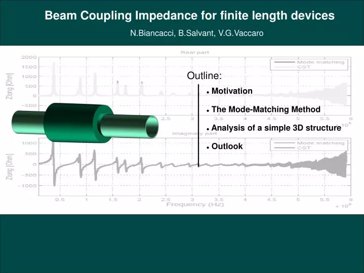
Beam Coupling Impedance for finite length devices. N.Biancacci, B.Salvant, V.G.Vaccaro. Outline: . Motivation The Mode-Matching Method Analysis of a simple 3D structure Outlook. Motivation. 1- Why finite length models?. Real life elements are finite in length

E N D
Beam Coupling Impedance for finite length devices N.Biancacci, B.Salvant, V.G.Vaccaro Outline: • Motivation • The Mode-Matching Method • Analysis of a simple 3D structure • Outlook
Motivation 1- Why finite length models? • Real life elements are finite in length • Usually 2D models are supposed to be enough accurate to obtain a quantitative evaluation of the beam coupling impedance • In case of segmented elements, or where the length becomes comparable with the beam transverse distance, this hypothesis could not work any more. • We suppose the image currents are passing through the surface of our element.
Mode Matching Method for Beam Coupling Impedance Computation Expansion of e.m. field in the waveguides by means of orthogonal wave modes radial waveguide waveguide cavity waveguide Representation of a circular cross section subdivided in subsets. radial waveguide Expansion of e.m. field in the cavity by means of an orthonormal set of eigenmodes Expansion of e.m. field in the radial waveguide by means of radial wave modes
ode Matching Method for Beam Coupling Impedance Computation Mode Matching Method for Beam Coupling Impedance Computation Cavity Eigenvector properties Divergenceless Eigenvectors (dynamic modes): In a more compact form the static modes may be considered as dynamic modes with kn=0. The Eigenvectors are always associated to a homogeneous boundary condition Irrotational Eigenvectors (static modes): The boundary condition are relevant to the tangential component of the Electric field.
Mode Matching Method for Beam Coupling Impedance Computation Explicit expressions for the cavity eigenvectors With: cavity αpis the pth zero of J0(αp)=0
Mode Matching Method for Beam Coupling Impedance Computation Explicit expressions of the e.m. fields in the cavity Remark:The unknown quantity is the matrix Ips
Mode Matching Method for Beam Coupling Impedance Computation Explicit expressions for waveguide modes Remark:The unknown quantities are the vectors V1pandV2p waveguides Where is the waveguide admittance of the p-mode and k0 is the free space propagation constant.
Mode Matching Method for Beam Coupling Impedance Computation Explicit expressions for the radial waveguide Remark:The unknown quantity is the vect or As In the above equation the boundary conditions are already satisfied at r=c and z=0,L. Where:εT is the dielectric constant in the torus, Radial waveguide
Mode Matching Method for Beam Coupling Impedance Computation Explicit expressions of the primary fields
Mode Matching Method for Beam Coupling Impedance Computation Matching conditions on the Magnetic fields Matching on the ports S1 and S2. 1 Matching on the torus inner surface. 2
Mode Matching Method for Beam Coupling Impedance Computation More involved is the matching of the Electric field because of the boundary conditions associated to the cavity eigenvectors. Namely the tangential component of the Electric field is strictly null on the entire close surface S.However we may obtain that the matching can be reached by means of non-uniform convergence of the eigenvector expansion. This can be achieved by an ad-hoc algebra of the expansion of the e.m fields.This will lead to the following expressions for the Ips coefficients. We have therefore 4 vector equations in 4 unknowns. The problem is in principle solvable.
Analysis of simple 3D Model A simple torus insertion will be used to study the effect of a finite length device on the impedance calculation.The Mode matching Method was applied to get the longitudinal impedance. c b 0 L z L To proof the reliability we set up 3 benchmarks: 1- Comparison with the classic thick wall formula for high values of sigma. 2- Comparisons with CST varying the conductivity. 3- Comparisons with CST varying the length. S3 S1 S2
1- Use of thick wall formula as a benchmark b=5cm c=30cm L=20cmεr=8
2- Crosscheck with CST – Varying σ (1/6) b=5cm c=30cm L=20cm εr=1 σ=10^-4
2- Crosscheck with CST – Varying σ (2/6) b=5cm c=30cm L=20cm εr=1 σ=10^-3
2- Crosscheck with CST – Varying σ (3/6) Increasing the scan step and magnifying, with the mode matching we can easily detectvery high resonances which may not look as they really are. ~1700Ω? b=5cm c=30cm L=20cm εr=1 σ=10^-3 ~21000Ω!
2- Crosscheck with CST – Varying σ (4/6) b=5cm c=30cm L=20cm εr=1 σ=1
2- Crosscheck with CST – Varying σ (5/6) b=5cm c=30cm L=20cm εr=1 σ=10^3
2- Crosscheck with CST – Varying σ (6/6) b=5cm c=30cm L=20cm εr=1 σ=10^4
3- Crosscheck with CST – Varying L (1/5) b=5cm c=30cm σ=10^-2 εr=1 L=20cm cut off
3- Crosscheck with CST – Varying L (2/5) b=5cm c=30cm σ=10^-2 εr=1 L=40cm
3- Crosscheck with CST – Varying L (3/5) b=5cm c=30cm σ=10^-2 εr=1 L=60cm
3- Crosscheck with CST – Varying L (4/5) b=5cm c=30cm σ=10^-2 εr=1 L=80cm
3- Crosscheck with CST – Varying L (5/5) b=5cm c=30cm σ=10^-2 εr=1 L=100cm
Conclusions The Torus model • We presented an application of the Mode Matching Method on a simple 3D model, a torus. • We successfully computed the longitudinal coupling impedance by means of this method. • A series of benchmarks, with analytical formulae and simulations, let us consider our analysis enough reliable: the comparison with the thick wall formula is in close agreement for high values of σ; the comparison with CST is in well agreement for the low conductivity case, increasing the conductivity they exhibit a different behavior. Outlook • Extend the model to compute the transverse impedances, dipolar and quadrupolar. • Compare the case of complex permittivity in CST. • Investigate the mismatch between CST and the Mode Matching code for high values of conductivity.