T-test for 2 Independent Sample Means

1. T-test for 2 Independent Sample Means Cohen Chap 7 – t-test for Independent samplemeans For EDUC/PSY 6600

2. We cannot solve problems by using the same kind of thinking that we used when we created them. Cohen Chap 7 – t-test for Independent sample means Albert Einstein

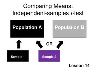
3. Intro • Same continuous DV compared across 2 independent (random) samples • Is there a significant difference between the 2 group means? • Do 2 samples come from different normal distributions with the same mean? • aka… • Independent-groups design • Between-subjects design • Between-groups design • Randomized-groups design Cohen Chap 7 – t-test for Independent sample means

4. Steps of a Hypothesis test “T-Test Statistic” • State the Hypotheses (Null & Alternative) • Select the Statistical Test & Significance Level • αlevel • One vs. Two tails • Select random samples and collect data • Find the region of Rejection • Based on α& # of tails • Calculate the Test Statistic • Examples include: z, t, F, χ2 • Make the Statistical Decision *even use z, if N > 100’ish

5. Separate Variance t-Test (need HOV) Steps of a Hypothesis test • State the Hypotheses (Null & Alternative) • Select the Statistical Test & Significance Level • αlevel • One vs. Two tails • Select random samples and collect data • Find the region of Rejection • Based on α& # of tails • Calculate the Test Statistic • Examples include: z, t, F, χ2 • Make the Statistical Decision Pooled-Variance t-Test (different sample sizes)

6. Example 1 • In order to assess the efficacy of a new antidepressant drug, 10 clinically depressed participants are randomly assigned to one of two groups. Five participants are assigned to Group 1, which is administered the antidepressant drug for 6 months. The other 5 participants are assigned to Group 2, which is administered a placebo during the same 6 month period • Assume that prior to introducing the treatments, the experimenter confirmed that the level of depression in the 2 groups was equal • After 6 months, all participants are rated by a psychiatrist (blind to participant assignment) on their level of depression

7. Example 1 library(tidyverse) library(furniture) ## Manually input data df <- data.frame(group1 = c(11, 1, 0, 2, 0), group2 = c(11, 11, 5, 8, 4)) ## Change to long form df_long <- df %>% tidyr::gather(key = "group", value = "value", group1, group2) ## Check Means and SD’s df_long %>% dplyr::group_by(group) %>% furniture::table1(value) df_long %>% ggplot(aes(x = group, y = value)) + geom_boxplot() group value [1] group1 11 [2] group1 1 [3] group1 0 [4] group1 2 [5] group1 0 [6] group2 11 [7] group2 11 ... ... ...

8. Example 1 - Output ────────────────────────────── group group1 group2 n = 5 n = 5 value 2.8 (4.7) 7.8 (3.3) ──────────────────────────────

9. Example 1 – T-Test df_long %>% car::leveneTest(value ~ group, data = ., center = "mean") #> Levene's Test for Homogeneity of Variance (center = mean) #> Df F value Pr(>F) #> group 1 .20 .667 #> 8 df_long %>% t.test(value ~ group, data = ., var.equal = TRUE) #> Welch Two Sample t-test #> data: value by group #> t = -1.9642, df = 7.1732, p-value = 0.08927 #> alternative hypothesis: true difference in means is not equal to 0 #> 95 percent confidence interval: #> -10.9900148 0.9900148 #> sample estimates: #> mean in group group1 mean in group group2 #> 2.8 7.8 Cohen Chap 7 – t-test for Independent sample means

10. Example 1 #> Levene's Test for Homogeneity of Variance (center = median) #> Df F value Pr(>F) #> group 1 0 1 #> 8 #> Welch Two Sample t-test #> data: value by group #> t = -1.9642, df = 8, p-value = 0.08511 #> alternative hypothesis: true difference in means is not equal to 0 #> 95 percent confidence interval: #> -10.8701282 0.8701282 #> sample estimates: #> mean in group group1 mean in group group2 #> 2.8 7.8 • After 6 months, the five participants taking the drug scored numerically lower on the depression scale (M = 2.80, SD = 4.66), compared their five counter parts taking placebo (M = 7.80, SD = 3.27). • To test the effectiveness of the drug at reducing depression, an independent samples t-test was performed. • The distribution of depression scores were sufficiently normal for the purposes of conducting a t-test (i.e. skew < |2.0| and kurtosis < |9.0|; Schmider, Sigler, Danay, Beyer, & Buhner, 2010). • Additionally, the assumption of homogeneity of variances was tested and satisfied via Levene’sF-test, F(4, 4) = .20, p = .667. • The independent samples t-test did not find a statistically significant effect, t(8) = -1.964, p = .085. • Thus, there is no evidence this drug reduces depression.

11. Assumptions (similar to 1-sample t-tests) • BOTH Samples were drawn INDEPENDENTLY at random (at least as representative as possible) Nothing can be done to fix NON-representative samples! Can not statistically test…violation: paired-samples t-test • The variable has a NORMAL distribution, for BOTH population Not as important if the sample is large (Central Limit Theorem) IF the sample is far from normal &/or small n, might want to transform variables Look at plots:histogram, boxplot, & QQ plot (straight 45º line)  sensitive to outliers!!! • Skewness & Kurtosis: Divided value by its SE & > ± 2 indicates issues • Shapiro-Wilks test (small N): p < .05  not normal • Kolmogorov-Smirnov test (large N): • HOV = Homogeneity of Variance: BOTH populations have the sample spread use Levene’s F-test (null= HOV)

12. Random Assignment • Random assignment to groups ↓ experimenter biases • Cases are enumerated • Numbers drawn and assigned to group in any of several ways • Does not ensure equality of group characteristics • Experiment: Random assignment & manipulation of IV • Treatment vs. control or 2 treatment groups • Quasi-experiment: Either randomization or manipulation • Non-experiment: Neither randomization or manipulation • Participants self-select or form naturally occurring groups Cohen Chap 7 – t-test for Independent sample means

13. Violations of assumptions • Equal groups: Violations ‘hurt’ less • Heterogeneity of variance • Small effects, p-value inaccurate ± .02 • Non-normality • Small effects, p-value inaccurate ± .02 • However: If samples are highly skewed or are skewed in opposite directions p-values can be *very* inaccurate • Both • Moderate effects if Nis large, p-value can be inaccurate • Large effects if Nis small, p-value can be *very* inaccurate Cohen Chap 7 – t-test for Independent sample means

14. Violations of assumptions • Unequal groups: Violations ‘hurt’ more • Heterogeneity of variance • Large effects • Non-normality • Large effects • Both • Huge effects • p-values can be **very** inaccurate with unequal ns and violations of assumptions, especially when Nis small Cohen Chap 7 – t-test for Independent sample means

15. Alternatives (assumptions violated) • Violation of normality or ordinal DV • Two Sample Wilcoxon test (aka, Mann-Whitney U Test) • Sample re-use methods • Rely on empirical, rather than theoretical, probability distributions • Exact statistical methods • Permutation and randomization tests • Bootstrapping Cohen Chap 7 – t-test for Independent sample means

16. Confidence Intervals • 95% CI for difference between means: μ1 - μ2 • Rearrange independent-samples t-test formula • Estimation as NHST (Null hypothesis Significance Test) • If H0: μ1 = μ2and if CI does NOT contain 0, reject H0 • If H0: μ1 = μ2 and if CI does contain 0, fail to reject H0 • Compute for in-class example Cohen Chap 7 – t-test for Independent sample means

17. Example 2 • An industrial psychologist is investigation the effects of different types of motivation on the performance of simulated clerical tasks. The 10 participants in the “individual motivation” sample are told that they will be rewarded according to how many tasks they successfully complete. The 12 participants in the “group motivation” sample are told that they will be rewarded according to the average number of tasks completed by all the participants in their sample. The number of tasks completed by each participant are as follows: • Individual Motivation: 11, 17, 14, 12, 11, 15, 13, 12, 15, 16 • Group Motivation: 10, 15, 4, 8, 9, 14, 6, 15, 7, 11, 13, 5 ──────────────────────────── group Individual Group n = 10 n = 12 value 13.6 (2.1) 9.8 (3.9) ──────────────────────────── ## data object is df2_long df2_long %>% dplyr::group_by(group) %>% furniture::table1(value)

18. Example 2 library(tidyverse) library(furniture) ## our data object is df2_long ## Check boxplots df2_long %>% ggplot(aes(x = group, y = value)) + geom_boxplot() Cohen Chap 7 – t-test for Independent sample means

19. Example 2 df2_long %>% car::leveneTest(value ~ group, data = ., center = "mean") #> Levene's Test for Homogeneity of Variance (center = "mean") #> Df F value Pr(>F) #> group 1 4.8287 0.03994 * #> 20 df2_long %>% t.test(value ~ group, data = ., var.equal = FALSE) #> Welch Two Sample t-test #> data: value by group #> t = 2.9456, df = 17.518, p-value = 0.008833 #> alternative hypothesis: true difference in means is not equal to 0 #> 95 percent confidence interval: #> 1.098587 6.601413 #> sample estimates: #> mean in group 1 mean in group 2 #> 13.60 9.75 Cohen Chap 7 – t-test for Independent sample means

20. Example 2 #> Levene's Test for Homogeneity of Variance (center = "mean") #> Df F value Pr(>F) #> group 1 4.8287 0.03994 * #> 20 #> Welch Two Sample t-test #> data: value by group #> t = 2.9456, df = 17.518, p-value = 0.008833 #> alternative hypothesis: true difference in means is not equal to 0 #> 95 percent confidence interval: #> 1.098587 6.601413sample estimates: #> mean in group 1 mean in group 2 #> 13.60 9.75 • The number of tasks completed was numerically higher among the individually motivated group (n = 10, M = 13.60, SD = 2.12), compared to the individuals being motivated by the groups results (n = 12, M = 9.75, SD = 3.89). • To test the difference in mean productivity, an independent samples t-test was performed. • The distribution of depression scores were sufficiently normal for the purposes of conducting a t-test (i.e. skew < |2.0| and kertosis < |9.0|; Schmider, Sigler, Danay, Beyer, & Buhner, 2010). • Additionally, the assumption of homogeneity of variances was tested and rejected via Levene’sF-test, F(9, 11) = 4.829, p = .040. • The independent samples, separate variances t-test found a statistically significant effect, t(17.52) = 2.946, p = .009. • Thus, individual motivation does result in a mean 3.85 additional tasks completed compared to group motivation (95% CI: [1.01, 6.60]).