Download
1 / 9
100 likes | 170 Views
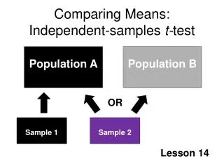
Chapter 10 T-test for independent means. Why? When you want to know if there are significant differences in characteristics (average income) between two independent groups (south/nonsouth). Example: page 164 Steps: 1. Null : No difference between Group 1 and 2

E N D
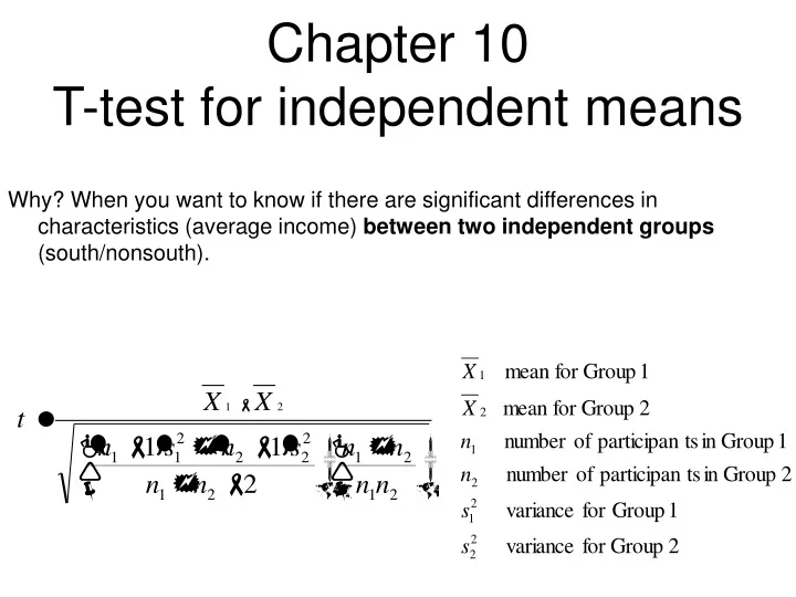
Chapter 10T-test for independent means Why? When you want to know if there are significant differences in characteristics (average income) between two independent groups (south/nonsouth).
Example: page 164 Steps: 1. Null: No difference between Group 1 and 2 Research: Difference between Group 1 and 2. • Set significance level: .05 • Select Appropriate test statistic: t-test independent samples (differences between different groups) • Compute test statistic (solve for t; do it by hand this time) • Determine value needed for rejection of null (find appropriate critical value in Table B2, Appendix B, p. 333)
determine degrees of freedom (df for this test-stat is n1- 1 + n2-1 or the sum of both groups (30+30=60) – 2, which is 58. • Find your df (58) and the appropriate significance level (.05) • The one tailed test is appropriate ONLY if the direction of the relationship is hypothesized (a directional-hypo; easier to pass a one-tailed test). 6. Compare critical (from table) and obtained value Obtained = -.14 and critical value is 2.001. Reject the null? • Do not reject null because the obtained value (-.14) does not exceed the critical value (2.001). Differences are probably due to random chance.
Using SPSS to conduct t-tests of independent samples • Get Troy’s state data • Analyze, compare means, independent-samples t-test • Click on income (adjincom) for test variable • Move grouping variable over to grouping variable box • Click define groups (and insert appropriate values) • Click okay or ok Another example: same thing comparing GOP controlled state gov’ts and others on % college educated.
Chapter 11t-tests: means of dependent groups • Dependent Samples – A t-test for dependent means indicates study of a single group of the same subjects. • The formula:
III. Same Steps (use new formula; use same table) Example: • Hypothetical: significant difference between state turnout rates with and without Perot in race? Steps for SPSS: • Analyze, compare means, paired-samples t-test • Move each variable over (e.g. pretest and posttest) • Click okay; interpret results.
Hypothesis Testing for a Difference Between ProportionsUse this procedure when you are trying to compare differences in the proportions (%s) between two groups. Where z is the z-scorep1 = proportion for group 1 (f1/n1)p2 = proportion for group 2 (f2/n2)n1=number in group 1n2=number in group 2p=total proportion (f1 + f2/n1 + n2)q=1-p
Example Are boys as likely to identify with their mother’s political party as girls? 85 boys and 70 girls were questioned and 34 of the boys and 14 of the girls identified with their mother’s political party. What can be concluded at the .05 level? Solution The hypotheses are H0: p1 = p2 (i.e., the proportion of boys identifying with their mother’s party is the same as that for girls). H1: p1 ≠ p2 (i.e., the proportion of boys identifying with their mother’s party is significantly different than that of girls). We have p1 = 34/85 = 0.4 p2 = 14/70 = 0.2 p = 48/155 = 0.31 q = 0.69
Evaluation: We are using a risk level of .05 (5% chance the null is true). That corresponds to a z-score of 1.65 (for a two-tailed test, see z table and figure 7.5, 124). Therefore, any obtained z-score that exceeds 1.65 is too extreme (improbable) to attribute to chance and the null must be rejected. This is ALWAYS the critical z-score for comparison with the obtained value. Clearly 2.68 is in the critical region, hence we can reject the null hypothesis and accept the alternative hypothesis and conclude that gender does make a difference for affiliation with mother’s party identification. Using SPSS (yes and no): Class example on gender and voting/pid.