Download
1 / 118
1.18k likes | 1.18k Views
Access the comprehensive documentation and examples of matplotlib for data fusion in .COMP.690. Explore the various plotting functions, tutorials, user's guide, and cookbook.

E N D
COMP 690 Data FusionMatplotlib Notes Albert Esterline Fall 2008
Documentation • Homepage http://matplotlib.sourceforge.net/ • Short descriptions of and links to documentation on all plotting functions • PyplotTutorial (8 pp.) http://matplotlib.sourceforge.net/users/pyplot_tutorial.html • Start here • Pyplot is a collection of command style functions that make matplotlib work like matlab • User’s Guide http://matplotlib.sourceforge.net/users_guide_0.98.3.pdf • Refer to as needed • Cookbook / Matplotlib http://www.scipy.org/Cookbook/Matplotlib • Lots of good examples • Shows figure, link to page giving code and explanation
Examples http://matplotlib.sourceforge.net/examples/ • Just a directory listing, but subdirectory names are descriptive • The “What's new” page http://matplotlib.sourceforge.net/users/whats_new.html • Every feature ever introduced into matplotlib is listed here under the version that introduced it • Often with a link to an example or documentation • Global Module Index http://matplotlib.sourceforge.net/modindex.html • Documentation on the various modules • This and the next are often the only places to find something • The Matplotlib API http://matplotlib.sourceforge.net/api/ • Documentation on the various packages
Matplotlib Backends • See http://matplotlib.sourceforge.net/api/index_backend_api.html • Matplotlib uses a backend to produce device-independent output (e.g., pdf, ps, png) • For backends without a GUI, only output is an explicitly-saved image file • File …\site-packages\matplotlib\mpl-data\matplotlibrc • sets the default backend with a line for the backend option • The Windows distribution has backend : TkAgg • Specifies the agg backend (for rendering) for Tkinter • Tkinter is a Python binding to the Tk GUI toolkit • Still the most popular Python GUI toolkit • Other toolkits: wxPython
Tk is an open source, cross-platform widget toolkit—library of basic elements for building a GUI • The antigrain geometry (Agg) library is a platform independent library • Provides efficient antialiased rendering with a vector model • Doesn't depend on a GUI framework • Used in web application servers and for generating images in batch scripts • Matplotlib includes its own copy of Agg • Aliasing is an effect that causes different continuous signals to become indistinguishable (aliases of one another) when sampled • Also refers to the resulting distortion • Anti-aliasing is the technique of minimizing this distortion • Used in digital photography, computer graphics, digital audio, etc.
matplotlib.pyplot vs. pylab • Package matplotlib.pyplot provides a MATLAB-like plotting framework • Package pylab combines pyplot with NumPy into a single namespace • Convenient for interactive work • For programming, it’s recommended that the namespaces be kept separate • See such things as import pylab • Or import matplotlib.pyplot as plt • The standard alias import numpy as np • The standard alias
Also from pylab import * • Or from matplotlib.pyplot import * from numpy import * • We’ll use from pylab import * • Some examples don’t show this—just assume it
Batch and Interactive Use • In a script, • import the names in the matplotlib namespace (pylab) • then list the commands Example: file E:\SomeFolder\mpl1.py from pylab import * plot([1,2,3,4]) show() • Executing E:\SomeFolder>mpl1.py produces the figure shown • The command line hangs until the figure is dismissed (click ‘X’ in the upper right)
plot() • Given a single list or array, plot() assumes it’s a vector of y-values • Automatically generates an x vector of the same length with consecutive integers beginning with 0 • Here [0,1,2,3] • To override default behavior, supply the x data: plot(x,y) where x and y have equal lengths show() • Should be called at most once per script • Last line of the script • Then the GUI takes control, rendering the figure
In place of show(), can save the figure to with, say, savefig(‘fig1.png’) • Saved in the same folder as the script • Override this with a full pathname as argument—e.g., savefig('E:\\SomeOtherFolder\\fig1.png') • Supported formats: emf, eps, pdf, png, ps, raw, rgba, svg, svgz • If no extension specified, defaults to .png
With the TkAgg backend, can use matplotlib from an arbitrary python (interactive) shell • Supposedly requires the matplotlibrc file to have interactive set to True (as well as backend to TkAgg ) • In the matplotlibrc file with the Windows distribution, the interactive setting (to False) is commented out • TkAgg sets interactive mode to True when show() or draw() executed • In batch mode (running scripts), interactive mode can be slow • Redraws the figure with each command.
Matplotlib from the Shell • Using matplotlib in the shell, we see the objects produced >>> from pylab import * >>> plot([1,2,3,4]) [<matplotlib.lines.Line2D object at 0x01A3EF30>] >>> show() • Hangs until the figure is dismissed or close() issued • show() clears the figure: issuing it again has no result • If you construct another figure, show() displays it without hanging
draw() • Clear the current figure and display a blank figure without hanging • Results of subsequent commands added to the figure >>> draw() >>> plot([1,2,3]) [<matplotlib.lines.Line2D object at 0x01C4B6B0>] >>> plot([1,2,3],[0,1,2]) [<matplotlib.lines.Line2D object at 0x01D28330>] • Shows 2 lines on the figure • Use close() to dismiss the figure and clear it • clf() clears the figure (also deletes the white background) without dismissing it • Figures saved using savefig() in the shell by default are saved in C:\Python25 • Override this by giving a full pathname
Interactive Mode • In interactive mode, objects are displayed as soon as they’re created • Use ion() to turn on interactive mode, ioff() to turn it off Example • Import the pylab namespace, turn on interactive mode and plot a line >>> from pylab import * >>> ion() >>> plot([1,2,3,4]) [<matplotlib.lines.Line2D object at 0x02694A10>] • A figure appears with this line on it • The command line doesn’t hang • Plot another line >>> plot([4,3,2,1]) [<matplotlib.lines.Line2D object at 0x00D68C30>] • This line is shown on the figure as soon as the command is issued
Turn off interactive mode and plot another line >>> ioff() >>> plot([3,2.5,2,1.5]) [<matplotlib.lines.Line2D object at 0x00D09090>] • The figure remains unchanged—no new line • Update the figure >>> show() • The figure now has all 3 lines • The command line is hung until the figure is dismissed
Matplotlib in Ipython • Recommended way to use matplotlib interactively is with ipython • In the Ipython drop-down menu, select pylab
Ipython’s pylab mode detects the matplotlibrc file • Makes the right settings to run matplotlib with your GUI of choice in interactive mode using threading • Ipython in pylab mode knows enough about matplotlib internals to make all the right settings • Plots items as they’re produce without draw() or show() • Default folder for saving figures on file C:\Documents and Settings\current user
Toolbar • In interactive mode, at the bottom left of the figure • Not included when a figure is written to file • From right to left Save: • Launches a file save dialog, initially at C:\Documents and Settings\current user with .png as default • All *Agg backends know how to save image types: PNG, PS, EPS, SVG Subplot configuration • Adjust the left, bottom, right, or top margin of the figure • With text, control spacing
The Zoom to rectangle: • Define a rectangle by • pressing the left mouse button to define one vertex and • dragging out to the opposite vertex and releasing • Content of the rectangle occupies the entire space for the figure The Pan/Zoom: 2 modes Pan Mode • Press the left mouse button, drag it to a new position • The figure is pulled along within the frame • Extended by blank area if needed Zoom Mode • Press the right mouse button, drag it to a new position • Figure is stretched proportional to the distance dragged in the direction dragged up and to the right. Shrunk proportional to the distance dragged down and to the left • Use modifier keys x, y or Ctrl to constrain the zoom to the x or y axis or to preserve the aspect ratio preserve, resp.
Forward and Back. • Navigate back and forth between previously defined views • Analogous to forward and back buttons of a web browser Home • Return to the first (default) view
More Curve Plotting • plot() has a format string argument specifying the color and line type • Goes after the y argument (whether or not there’s an x argument) • Can specify one or the other or concatenate a color string with a line style string in either order • Default format string is 'b-' ( solid blue line) • Some color abbreviations b (blue), g (green), r (red), k (black), c (cyan) • Can specify colors in many other ways (e.g., RGB triples) • Some line styles that fill in the line between the specified points - (solid line), -- (dashed line), -. (dash-dot line), : (dotted line) • Some line styles that don’t fill in the line between the specified point o (circles), + (plus symbols), x (crosses), D (diamond symbols) • For a complete list of line styles and format strings, http://matplotlib.sourceforge.net/api/pyplot_api.html#module-matplotlib.pyplot • Look under matplotlib.pyplot.plot()
The axis() command takes a list [xmin, xmax, ymin, ymax] and specifies the view port of the axes Example In [1]: plot([1,2,3,4], [1,4,9,16], 'ro') Out[1]: [<matplotlib.lines.Line2D object at 0x034579D0>] In [2]: axis([0, 6, 0, 20]) Out[2]: [0, 6, 0, 20]
Other arguments for the axis() command • ‘off’ turns off the axis lines and labels • ‘equal’ changes the limits of the x and y axes so that equal increments of x and y have the same length • ‘scaled’ achieves the same result as ‘equal’ by changing the dimensions of the plot box instead of the axis limit • ‘tight’ changes the axis limits to show all the data and no more • ‘image’ is scaled with the axis limits equal to the data limits • axis() with no argument returns the current axis limits, [xmin, xmax, ymin, ymax]
Generally work with arrays, not lists • All sequences are converted to NumPy arrays internally • plot() can draw more than one line at a time • Put the (1-3) arguments for one line in the figure • Then the (1-3) arguments for the next line • And so on • Can’t have 2 lines in succession specified just by their y arguments • matplotlib couldn’t tell whether it’s • a ythen the next yor • an xthen the corresponding y • The example (next slide) illustrates plotting several lines with different format styles in one command using arrays
In [1]: t = arange(0.0, 5.2, 0.2) In [2]: plot(t, t, t, t**2, 'rs', t, t**3, 'g^') Out[2]: [<matplotlib.lines.Line2D object at 0x02A6D410>, <matplotlib.lines.Line2D object at 0x02A6D650>, <matplotlib.lines.Line2D object at 0x02A6D8D0>]
If the y for plot() is 2-dimensional, then the columns are plotted—e.g., In [1]: a = linspace(0, 2*pi, 13) In [2]: b_temp = array([sin(a), cos(a)]) In [3]: b = b_temp.transpose() In [4]: plot(a, b) Out[4]: [<matplotlib.lines.Line2D object at 0x02A770D0>, <matplotlib.lines.Line2D object at 0x02A77150>]
Controlling Line Properties • Lines you encounter are instances of the Line2D class • Instances have the following properties alpha = 0.0 is complete transparency, alpha = 1.0 is complete opacity
Markers • Some of the line types in a format string give continuous lines • A marker is a symbol displayed at only the specified points on a continuous line • In the format string, indicate a marker with a 3rd symbol • One of +, o, s, v, x, >, <, ^ • The 3 symbols can occur in any order • No ambiguity: a marker can’t be used with a non-continuous line type In [50]: plot([0,1,2,3], 'g:o') Out[50]: [<matplotlib.lines.Line2D object at 0x03017BB0>]
Three Ways to Set Line Properties • One way: Use keyword line properties as keyword arguments—e.g., plot(x, y, linewidth=2.0) • Another way: Use the setter methods of the Line2D instance • For every property prop, there’s a set_prop() method that takes an update value for that property • To use this, note that plot() returns a list of lines—e.g., line1, line2 = plot(x1,y1,x2,x2) • The following example has 1 line with tuple unpacking line, = plot(x, y, 'o') line.set_antialiased(False)
The 3rd (and final) way to set line properties: use function setp() • 1st argument can be an object or sequence of objects • The rest are keyword arguments updating the object’s (or objects’) properties • The following sets the color and linewidth properties of two lines lines = plot(x1, y1, x2, y2) setp(lines, color='r', linewidth=2.0) • setp() also accepts property-value pairs of arguments with property names as strings—e.g., setp(lines, 'color', 'r', 'linewidth', 2.0)
When setp() has just an object and a property name as arguments, it lists all possible values for that property In [38]: setp(l1, 'linestyle') linestyle: [ '-' | '--' | '-.' | ':' | 'steps' | 'steps-pre' | 'steps-mid' | 'steps-post' | 'None' | ' ' | '' ] • When setp() has an object as its sole argument, it lists the names of the properties of that object
Multiple Figures and Axes • Pylab has the concepts of the current figure and the current axes • An instance of class Figure contains all the plot elements • An instance of class Axes contains most of the figure elements: instances of Axis, Tick, Line2D, Text, Polygon, … • But 1 figure may have multiple instances of Axes (“graphs”) • All plot and text label commands apply to the current axes • Function gca() returns the current axes as an Axes instance • Function gcf() returns the current figure as a Figure instance • Normally, all is taken care of behind the scenes
Function figure() returns an instance of Figure • Can take a number of arguments • Most have reasonable defaults set in the matplotlibrc file • Typically called with 1 (the figure number) or none • Called with none, the figure number is incremented and a new, current figure returned • The figure number starts at 1 • A Figure instance has a number property • Called with an integer argument, • if there’s a figure with that number, it becomes the current figure • If not, a new figure with that number is created
Example using multiple figures figure(1) plot([1,2,3]) figure(2) plot([4,5,6]) figure(1) # make figure 1 current title('Easy as 1,2,3') • In ipython, this opens 2 figure windows
Now consider close() more generally • Takes 1 or no argument; if the argument is • None, closes the current figure • A number, closes the figure with that number • A Figure instance, closes that figure • ‘all’, closes all figures
Text • The text commands are self-explanatory • xlabel() • ylabel() • title() • text() • In simple cases, all but text() take just a string argument • text() needs at least 3 arguments: x and y coordinates (as per the axes) and a string • All take optional keyword arguments or dictionaries to specify the font properties • They return instances of class Text
plot([1,2,3]) xlabel('time') ylabel('volts') title('A line') text(0.5, 2.5, 'Hello world!')
Three ways to specify font properties: using • setp • object oriented methods • font dictionaries Controlling Text Properties with setp • Use setp to set any property t = xlabel('time') setp(t, color='r', fontweight='bold') • Also works with a list of text instances • E.g., to change the properties of all the tick labels labels = getp(gca(), 'xticklabels') setp(labels, color='r', fontweight='bold')
Controlling Text Using Object Methods • setp is just a wrapper around the Textset methods • Can prepend set_ to the text property and make a normal instance method call t = xlabel('time') t.set_color('r') t.set_fontweight('bold')
Controlling Text Using Keyword Arguments & Dictionaries • All text commands take an optional dictionary argument and keyword arguments to control font properties • E.g., to set a default font theme and override individual properties for given text commands font = {'fontname' : 'Courier', 'color' : 'r', 'fontweight' : 'bold', 'fontsize' : 11} plot([1,2,3]) title('A title', font, fontsize=12) text(0.5, 2.5, 'a line', font, color='k') xlabel('time (s)', font) ylabel('voltage (mV)', font)
Legends • A legend is a box (by default in upper right) associating labels with lines (displayed as per their formats) legend(lines, labels) where lines is a tuple of lines, labels a tuple of corresponding strings from pylab import * lines = plot([1,2,3],'b-',[0,1,2],'r--') legend(lines, ('First','Second')) savefig('legend')
If there’s only 1 line, be sure to include the commas in the tuples lengend((line1,), (‘Profit’,)) • Use keyword argument loc to override the default location • Use predefined strings or integer codes ‘upper right’ 1 ‘upper left’ 2 ‘lower left’ 3 ‘lower right’ 4 ‘right’ 5 ‘center left’ 6 ‘center right’ 7 ‘lower center’ 8 ‘upper center’ 9 ‘center’ 10 • E.g., legend((line,), (‘Profit’,) , loc=2)
Writing Mathematical Expressions • Can use TeX markup in any text element • For usage, requirements, backend info, see mathtext documentation http://matplotlib.sourceforge.net/api/mathtext_api.html • Use raw strings (precede the quotes with an 'r') • Surround the string text with $’s (as in TeX) title(r'$\alpha > \beta$') • Regular text and mathtext can be interleaved within the same string • To make subscripts and superscripts use '_' and '^‘—e.g., title(r'$\alpha_i > \beta_i$')
Can use many TeX symbols, e.g., \infty, \leftarrow, \sum, \int • The over/under subscript/superscript style is supported • E.g., to write the sum of xi, i from 0 to , text(1, -0.6, r'$\sum_{i=0}^\infty x_i$') • Default font is italics for mathematical symbols • To change fonts, e.g., to write “sin” in Roman, enclose the text in a font command—e.g., text(1,2, r's(t) = $\mathcal{A}\mathrm{sin}(2 \omega t)$') • Many commonly used function names typeset in a Roman font have shortcuts • The above could be written as text(1,2, r's(t) = $\mathcal{A}\sin(2 \omega t)$')
Font choices Roman \mathrm italics \mathit caligraphy \mathcal typewriter \mathtt • Accents : \hat, \breve, \grave, \bar, \acute, \tilde, \vec, \dot, \ddot • E.g., overbar on an “o”: \bar{o}
from pylab import * t = arange(0.0, 2.0, 0.01) s = sin(2*pi*t) plot(t,s) title(r'$\alpha_i > \beta_i$', fontsize=20) text(1, -0.6, r'$\sum_{i=0}^\infty x_i$', fontsize=20) text(0.6, 0.6, r'$\mathcal{A}\mathrm{sin}(2 \omega t)$', fontsize=20) xlabel('time (s)') ylabel('volts (mV)') savefig('mathtext_tut', dpi=50)
Axes Properties • There’s a current instance of Axes in the current figure • Contains all the graphical elements • gca() returns the current instance of Axes • cla() clears it • The following are a few get_ methods, all with no arguments • Most self-explanatory get_legend() get_lines() get_title()
For the x axis get_xlabel() get_xbound() • Returns the x-axis numerical bounds in the form of a tuple (lbound, ubound) get_xlim() • Like get_xbound(), but returns an array • Similar get_ methods for the y axis • Corresponding commands for setting Axes properties • Use object methods (set_) or setp() • If a 2-element tuple or array is returned, method takes 2 corresponding arguments
Grids • Use grid() function or grid() Axes method • With no arguments, gives a dotted black line at each tick on both axes • To suppress the grid, use grid(None) • Or simply grid() when there’s already a grid • Takes keyword arguments grid(color='r', linestyle='-', linewidth=2) • Axes get_ methods get_xgridlines() get_ygridlines() • Corresponding set_ methods, or use setp()