Download
1 / 26
260 likes | 444 Views
PSY 307 – Statistics for the Behavioral Sciences. Chapter 13 – Single Sample t-Test Chapter 15 -- Dependent Sample t-Test. Midterm 2 Results. The top score on the exam and for the curve was 58 – 4 people were close to it. Student’s t-Test.

E N D
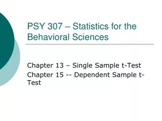
PSY 307 – Statistics for the Behavioral Sciences Chapter 13 – Single Sample t-Test Chapter 15 -- Dependent Sample t-Test
Midterm 2 Results The top score on the exam and for the curve was 58 – 4 people were close to it.
Student’s t-Test • William Sealy Gossett published under the name “Student” but was a chemist and executive at Guiness Brewery until 1935.
What is the t Distribution? • The t distribution is the shape of the sampling distribution when n < 30. • The shape changes slightly depending on the number of subjects. • The degrees of freedom (df) tell you which t distribution should be used to test your hypothesis: • df = n - 1
Comparison to Normal Distribution • Both are symmetrical, unimodal, and bell-shaped. • When df are infinite, the t distribution is the normal distribution. • When df are greater than 30, the t distribution closely approximates it. • When df are less than 30, higher frequencies occur in the tails for t.
The Shape Varies with the df (k) Smaller df produce larger tails
Comparison of t Distribution and Normal Distribution for df=4
Finding Critical Values of t • Use the t-table NOT the z-table. • Calculate the degrees of freedom. • Select the significance level (.05, .01). • Look in the column corresponding to the df and the significance level. • If t is greater than the critical value, then the result is significant (reject the null hypothesis).
Link to t-Tables http://www.statsoft.com/textbook/sttable.html
Calculating t • The formula for t is the same as that for z except the standard deviation is estimated – not known. • Sample standard deviation (s) is calculated using (n – 1) in the denominator, not n.
Confidence Intervals for t • Use the same formula as for z but: • Substitute the t value (from the t-table) in place of z. • Substitute the estimated standard error of the mean in place of the calculated standard error of the mean. • Mean ± (tconf)(sx) • Get tconf from the t-table by selecting the df and confidence level
Assumptions • Use t whenever the standard deviation is unknown. • The t test assumes the underlying population is normal. • The t test will produce valid results with non-normal underlying populations when sample size > 10.
Deciding between t and z • Use z when the population is normal and s is known (e.g., given in the problem). • Use t when the population is normal but s is unknown (use s in place of s). • If the population is not normal, consider the sample size. • Use either t or z if n > 30 (see above). • If n < 30, not enough is known.
What are Degrees of Freedom? • Degrees of freedom (df) are the number of values free to vary given some mathematical restriction. • Example – if a set of numbers must add up to a specific toal, df are the number of values that can vary and still produce that total. • In calculating s (std dev), one df is used up calculating the mean.
Example • What number must X be to make the total 20? 5 100 10 200 7 300 X X 20 20 Free to vary Limited by the constraint that the sum of all the numbers must be 20 So there are 3 degrees of freedom in this example.
A More Accurate Estimate of s • When calculating s for inferential statistics (but not descriptive), an adjustment is made. • One degree of freedom is used up calculating the mean in the numerator. • One degree of freedom must also be subtracted in the denominator to accurately describe variability.
Within Subjects Designs • Two t-tests, depending on design: • t-test for independent groups is for Between Subjects designs. • t-test for paired samples is for Within Subjects designs. • Dependent samples are also called: • Paired samples • Repeated measures • Matched samples
Examples of Paired Samples • Within subject designs • Pre-test/post-test • Matched-pairs
Dependent Samples • Each observation in one sample is paired one-to-one with a single observation in the other sample. • Difference score (D) – the difference between each pair of scores in the two paired samples. • Hypotheses: • H0: mD = 0 mD ≤ 0 • H1: mD ≠ 0 mD > 0
Repeated Measures • A special kind of matching where the same subject is measured more than once. • This kind of matching reduces variability due to individual differences.
Calculating t for Matched Samples • Except that D is used in place of X, the formula for calculating the t statistic is the same. • The standard error of the sampling distribution of D is used in the formula for t.
Degrees of Freedom • Subtracting values for two groups gives a single difference score. • The differences, not the original values, are used in the t calculation, so degrees of freedom = n-1. • Because observations are paired, the number of subjects in each group is the same.
Confidence Interval for mD • Substitute mean of D for mean of X. • Use the tconf value that corresponds to the degrees of freedom (n-1) and the desired a level (e.g., 95%= .05 two tailed). • Use the standard deviation for the difference scores, sD. • Mean D ± (tconf)(sD)
When to Match Samples • Matching reduces degrees of freedom – the df are for the pair, not for individual subjects. • Matching may reduce generality of the conclusion by restricting results to the matching criterion. • Matching is appropriate only when an uncontrolled variable has a big impact on results.
Deciding Which t-Test to Use • How many samples are there? • Just one group -- treat as a population. • One sample plus a population is not two samples. • If there are two samples, are the observations paired? • Do the same subjects appear in both conditions (same people tested twice)? • Are pairs of subjects matched (twins)?