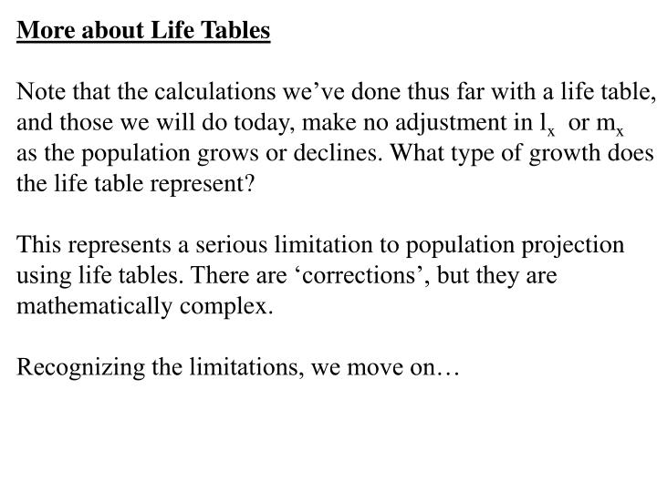
More about Life Tables Note that the calculations we’ve done thus far with a life table,

More about Life Tables Note that the calculations we’ve done thus far with a life table, and those we will do today, make no adjustment in lx or mx as the population grows or declines. What type of growth does the life table represent? This represents a serious limitation to population projection using life tables. There are ‘corrections’, but they are mathematically complex. Recognizing the limitations, we move on…

From lx, mx (in Ricklefs’ text fecundity is ‘bx’), and age class information, you can calculate an approximate (but usually quite accurate) value for “r”. The method is shown in the supplement, but we’ll go through our life table to demonstrate it here. After calculating R0, calculate and sum x lxmx. survivorship fecundity Age class lx bx lxbx x lxbx 0 1.0 0.0 0 0 1 .8 0.2 0.16 0.16 2 .6 0.3 0.18 0.36 3 .4 1.0 0.4 1.2 4 .4 0.6 0.24 0.96 5 .2 0.1 0.02 0.10 6 0 ---- ----- R0 = 1.0  = 2.78

Divide Σxlxmx by R0 . What you have calculated is the age-weighted mean of the distribution of births by age. It’s the equivalent of finding the age at which you could balance a cutout of the distribution on a ruler. In physics this is called the first moment of the distribution. My guess... bx age

The quotient is an estimate of the generation time for this species/life table. The generation time is usually called either T (in Ricklefs’ text) or G (most other texts).  x lxbx = 2.78 R0 = 1.0  x lxbx /R0 = 2.78/1.0 = 2.78 = T Now go back to the basic equation for continuous exponential growth… Nt = N0 ert or Nt/N0 = ert if we set the time t as one generation time, we know the values of most of the terms in the equation...

Since the time is one generation, we know that the ratio Nt/N0 is the net replacement rate. Thus, the equation becomes: Nt/N0 = R0 = erT Now take the logs of both sides of the equation… ln (R0) = rT ln (1.0) = r (2.78) 0 = 2.78r r = 0

We already “knew” this result, i.e. that if R0 was 1, then r = 0. But we also modified the initial life table to show that small change in survivorship and/or reproduction could lead to growth or decline in the population. Let’s re-calculate again for the modified life table (m3 = 0.6 in the original table). Age class lx bx lxbx xlxbx 0 1.0 0.0 0 0 1 .8 0.2 0.16 0.16 2 .6 0.3 0.18 0.36 3 .4 1.0 0.4 1.2 4 .4 1.0 0.4 1.6 5 .2 0.1 0.02 0.10 6 0 ---- ----- R0 = 1.16 = 3.42

Making the same calculations: T = 3.42/1.16 = 2.95 r = ln R0 /T = ln (1.16)/2.95 r = 0.148/2.95 = 0.05 An “r” > 0 indicates that this population is growing, but we knew that because R0 was >1. Finally (to guild the lily) let’s see what happens if survivorship and/or reproduction is less than the values producing an R0 = 1. (by changing l4 and m4.)…

Age class lx bx lxbx x lxbx 0 1.0 0.0 0 0 1 .8 0.2 0.16 0.16 2 .6 0.3 0.18 0.36 3 .4 1.0 0.4 1.2 4 .3 0.4 0.12 0.48 5 .2 0.1 0.02 0.10 6 0 ---- ----- R0 = 0.88 = 2.10 T = 2.10/0.88 = 2.386 r = ln(0.88)/2.386 r = -0.128/2.386 = -.053 R is < 1, and “r” is negative. This population is declining.

The life table uses fixed, constant values for survivorship and natality. Is there evidence of density-dependence in the life table? No! So, how is a density response evident? There must be a change in either the birth rate or the death rate as density changes. Remember that r = b – d. A change in either will change the population growth rate. There are matrix methods to put density dependence into a form of the life table, changing lx and bx with density , but they are beyond the scope of this course.

If the change is a general one in the pattern of birth and/or death rate, the carrying capacity K will change, as well as the observed rate of increase at any density. For example, Peregrine falcons exposed to DDT had a much reduced reproductive success due to egg shell thinning. This is what it might look like:

Alternatively, excessive harvesting might have its effect on death rates. This, too, would change the K and the observed growth rate at any density. This certainly happened to a variety of whale species.

Here’s a neat experiment showing density dependence: Eisenberg, working in a pond only a few miles from here, showed that egg production in snails is density-dependent. He established 3 kinds of populations, each in a separate enclosure, along the edges of the pond: 1. high density (an experimental treatment produced by increasing egg density by 5x) 2. low density (this experimental treatment produced by reducing the density of eggs to 1/5 of control) 3. control (natural egg density) The snails grew from these eggs, and he measured egg production in the three treatments…

There were naturally about 1000 eggs within each enclosed area. Eggs were moved from low density (LD) areas into high density (HD) areas, bringing the total number of eggs at HD to ~5000, and reducing the number in LD areas to ~200. C LD Diagram of the pond with fenced enclosures along the shore. HD

After the snails grew, egg production at high density (5000 snails/m2) was reduced to about 10% of that in treatments at low density (200 snails/m2). That difference in fecundity brought the numbers of eggs in all three treatments to very similar levels – density compensation. In snails, egg production depends on food quality. They scrape food from the surfaces of plants in the pond. plants protein egg production Eisenberg added a 6 oz. package of frozen spinach to a few groups. Their egg production was about 10x controls, even though the quantitative increase in amount of plant was miniscule. Food quality!! Density-dependence!!

Remember again the critical problems with the exponential growth model… Basically, they involve a lack of realism. Natural populations are limited by both biological and physical conditions in the environment. Physical conditions include climatic extremes (seasonality, storms, etc.), drought, and other factors. Biological conditions such as competition and predation also limit population growth. They are the subject of much of the second half of the course.

Whatever the causes, there is evidence of density dependence even in the growth of the U.S. population… Evidence that growth slows as carrying capacity is approached: 1) Human population growth in the United States… as population size has increased, the intrinsic rate of increase has slowed...

However, more recent censuses indicate that there has been a change since that 1910 census. Growth hasn’t continued to slow as much as the graph plotting effective r indicated.

2) Evidence of the impact of habitat quality in limiting population growth. Remember that r = b - d. Anything that causes birth rate to decline or death rate to increase will decrease little r. Anything that leads to a lower value for K should cause a population to respond in life history values. In a population of white-tailed deer in New York State, habitat quality and statistics indicating birth rate clearly indicate the linkage… Region % pregnant embryos Western (best) 94 1.71 Central (intermediate) 87 1.37 Adirondack (worst) 79 1.06

Some other examples: In Drosophila lifespan declines at high density, but there is a decrease in fecundity beginning at much lower densities…

In song sparrows on Mendarte Island off the BC coast… Males are territorial. As population density increases, there are more males that don’t hold territories and can’t breed successfully. The number of young fledged per female decreases with density, and… The percentage of juveniles (fledged) decreases as the autumn adult population increases.

Finally, as plant density increases, the size of individual plants decreases. Since the number of seeds produced by a plant (a preliminary measure of its fitness) is basically proportional to its biomass (size), decreasing plant size indicates a key density response that will tend to limit the plant’s population size. This is for flax…

The equation for the logistic model can be manipulated to demonstrate other aspects of the predictions… dN/dt = rN (1 - N/K) 1/N dN/dt = r (1 - N/K) now we have an equation for growth rate per head. Note that it is a linear equation, where the per head growth rate drops from r to 0 as the population grows toward K.

The way in which dN/dt changes with increasing population size is also important. It dictates the population size that can be most effectively harvested, i.e. when the population will grow most rapidly to replace harvested individuals… dN/dt = rN (1 - N/K) = rN - rN2/K this is the equation of an inverted parabola, with the maximum value of dN/dt indicated by a 0 in the derivative of this equation with respect to N… 0 = r - 2rN/K r = 2rN/K K = 2N N = K/2

Review summarizing density-dependence thus far: • For most natural species density-dependence is evident in • birth and/or death rates • As N increases, typically birth rates decrease and death • rates increase • These changes are reflected in the growth rate, and keep • population size close to K

All this is described as negative density-dependence, since the rate of population growth decreases as population size increases. • However… • There are certain conditions that can lead to positive density-dependence, particularly when a population is small: • When a population is very small, mate finding may be • difficult. Therefore, the birth rate at low density is far lower than the simple logistic model projects. This is called the Allee effect. Very small (frequently rare, endangered species) populations dwindle toward or to extinction.

2) Small populations may also suffer from genetic inbreeding. Inbreeding exposes the presence of deleterious mutations in offspring, reducing their fitness. Fitness reduction means that these individuals are likely to produce fewer offspring, and the population will decline. Increasing population size decreases inbreeding and leads to a higher growth rate – a positive density- dependence – but only in the increase from very small population size that causes high inbreeding. Then negative density-dependence takes over again. This happened in Florida panthers and may be happening in the African cheetah. Evidence?

Florida panthers (Felis concolor) are highly endangered. In the 1980s the total population was <50 individuals with an effective population size of ~25. They occurred in two main groups: One group in the Everglades, and the other further north, but with limited contact between them.

In these small populations inbreeding occurred. Molecular evidence of the inbreeding became apparent from low genetic variation in microsatellite loci. Inbreeding also exposed a number of deleterious traits (appearing in homozygous recessives): A kinked tail A ‘cowlick’ of fur over the shoulders Males are cryptorchid (only one testicle descends A high proportion of defective sperm (also kinked ‘tails’) Genetic rescue, introducing some Texas panthers (same species but different subspecies) creates the likelihood of outbreeding and has been relatively successful since 2000.

In the case of the cheetah, humans have only had limited impact on a long-term loss of genetic diversity. Cheetahs today are remarkable in the low genetic diversity evident in comparisons of protein and nuclear markers. What has this meant for cheetahs?

One more complication… The basic logistic model predicts smooth growth to an equilibrium population size, K. There are reasons to question the simplicity of that model. One source of complication: it assumes that each individual contributes to further population growth beginning at birth. Is that realistic? No! Correcting that assumption means adding time lags to the model. There are 2 basic forms of lag… a gestation time lag - the time between conception and birth a maturation time lag - the time between birth and reproductive maturity

Time lags lead to oscillations in population size… As a population approaches K, time lags cause a reproductive response appropriate for an earlier, smaller population Depending on the amount of growth that occurs during the lag time, the result can be a population with damped oscillations that eventually lead to a stable equilibrium, or one that undergoes continuing, pernicious oscillations until extinction. Since the result depends on growth during lag, high “r” leads to high amplitude oscillation long lag leads to high amplitude oscillation

You can generate oscillating population dynamics using Populus. Try the following parameters to get damped oscillation: N0 = 5, K = 500, r = 0.2, T = 2 and try these values to get “pernicious” oscillations that would lead to likely extinction: N0 = 5, K = 500, r = 0.5, T = 5 if you were to increase the r in the last set of parameters to 1, you get a single, large oscillation.

Here is a figure that shows you how the oscillations change with the product rτ:

Reviewing the other assumptions of the logistic model: 1) The population structure is homogeneous…there is no age structure or individual variation in size and resource use. 2) All have the same birth and death rates. Earlier this was described as all individuals having identical life histories. This also obviates sex. 3) K is a constant…the quality of the environment does not change over time. So is r. Not only are their life histories identical, but they don’t change with density or over time. 4) There are no time lags.

How useful is the logistic in describing the growth of real populations? It works reasonable well for some species with simple life cycles, generally those with short lifespans as well. It also works for additional species when growth occurs under strictly controlled laboratory conditions. In the “real” world, however, most species have: 1)either high r or long enough time lags to produce, if not cycles, growth which does not fit the simple logistic well. 2)exposure to a changing environment, and thus a changing K. 3)apparently stochastic dynamics

To show you how well the logistic can fit real data, here’s a classic growth curve for E. coli:

And here’s one that shows you how dramatically a change in temperature can alter the carrying capacity for a growing population. These are growth curves for Drosophila melanogaster. How could the growth curve look logistic if the temperature keeps varying?

More about Life Tables Note that the calculations we’ve done thus far with a life table,