Download
1 / 20
200 likes | 420 Views
Assessing the skill of an all-season statistical forecast model of the Madden-Julian Oscillation. Xian-an Jiang, Duane E. Waliser Jet Propulsion Laboratory/California Institute of Technology, Pasadena, CA Matthew C. Wheeler Bureau of Meteorology Research Centre, Melbourne, Australia

E N D
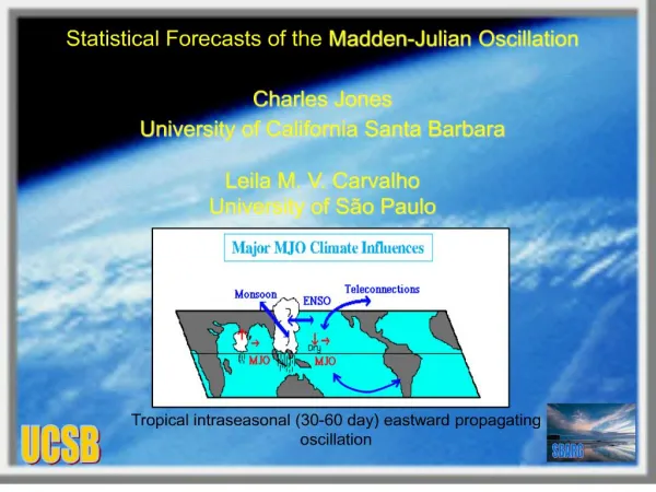
Assessing the skill of an all-season statistical forecast model of the Madden-Julian Oscillation Xian-an Jiang, Duane E. Waliser Jet Propulsion Laboratory/California Institute of Technology, Pasadena, CA Matthew C. Wheeler Bureau of Meteorology Research Centre, Melbourne,Australia Charles Jones Institute for Computational Earth System Science, UCSB, CA Myong-In Lee, and Siegfried D. Schubert Global Model and Assimilation Office, NASA/GSFC, MD
Motivation: Why Subseasonal Variability / Madden-Julian Oscillation? • Provide a more realistic benchmark for numerical forecast models; • Provide assessment of a statistical model for the real-time forecast of the MJO; • …seenext page Weather (~days) Interannual (~seasons) Subseasonal (~weeks) Why empirical model? Dynamical models: skill only up to lead times of about 7-10days. (e.g., Waliser et al.,1999, 2004; Hendon et al.,2000; Jones et al, 2000;Seo et al, 2005; andothers.) Empirical models:15 days (rainfall/OLR), 20-25days for dynamical fields. (e.g., von Storch and Xu,1990; Waliser et al.,1999; Lo and Hendon, 2000;Jones et al., 2004; Wheeler and Weickmann, 2001; Mo, 2001; and others) Why current study (real-time scheme; Wheeler and Hendon 2004)? ? Real-time application Time-filtering
Motivation (cont’d) Hybrid Forecast: Empirical + Dynamical • Provide a near-term means to improve extended-range predictions; • Motivate the need to improve intrinsic capability in MJO prediction in the dynamical models.
Model construction (I) MJO Index EOF 1 (11%) Combined EOF (OLR,u850, u200) (15oS-15oN ; Wheeler and Hendon 2004) NCEP-DOE2 Reanalysis Daily, 1983-2004 • Annual cycle removed; • Interannual variability (ENSO) removed: • Regression pattern of each variable against the PC of SST rotated EOF1 (ENSO); • 120-day mean of previous 120 days. EOF 2 (10%)
Model construction (II) Time series of Combined EOF PC1 PC2 Combined Amplitude Strong MJO Weak MJO
Model construction (III) Lagged regression Model Time at forecast point: t0 Variable A at particular grid point at forecast lead ndt: A(x,y,p,t0+ndt) A(x,y,p,t0+ndt) = reg1(x,y,p,ndt) × PC1(t0) + reg2(x,y,p,ndt) × PC2(t0) reg1(x,y,p,ndt) andreg2(x,y,p,ndt): • Based on historical observations • Seasonal dependent KEY: How to get PC1(t0) and PC2(t0) (the real-time MJO index)?
Real-time forecast flow chart Remove Project to SST EOF1 SST’ SST PCsst annual cycle Regression pattern to PCsst based on historical dataset Real-time Observations at t0 IAV of OLR, u850,u200 Remove IAV OLR, u850,u200 OLR’*, u850’*,u200’* OLR’, u850’,u200’ Remove annual cycle Remove previous 120-day mean Project to CEOF 1 & 2 reg1(x,y,p,ndt),reg2(x,y,p,ndt) Lag Regression Forecast Model PC1(t0), PC2(t0) Lag Regression pattern for each variable against PC1 & 2 based on historical dataset A(x,y,p,t0+ndt) A: u, v, t, q & OLR, SLP.
Cross-validation: 1 1983 1984 1985 1986 …... …... …... 2002 2003 2004 Construct lag-regression coefficients Forecast/validation 1983 1984 1985 1986 …... …... …... 2002 2003 2004 2 …….. ….. 21 1983 1984 1985 …... 2001 2002 2003 2004 22 1983 1984 1985 …... 2001 2002 2003 2004 Forecast starting date: 1st, 6th, 11th, 16th, 21st, and 26th of each month. Summer: Forecasts with the starting date during Jun, Jul, Aug. Winter: Nov, Dec and Jan.
Predictive Skills Pattern correlation (Forecast vs EOF filtered Observations) (30oS-30oN, global longitudes) OLR 0.36 0.19
Temporal Correlation (against EOF filtered OBS) OLR 5d 10d 15d 20d
Correlation (vs. unfiltered OBS) Winter 850mb u-wind OLR 5d 10d 15d 20d
Correlation (vs. unfiltered OBS) 200mb u-wind Winter 5d 10d 15d 20d
Sensitivity Tests (I) Advantage by using seasonal-dependent regression coefficients
Sensitivity Tests (II) Including more PCs in the regression model Summer Winter 2PCs 5PCs
Sensitivity Tests (III) More lagged information in the regression model
Sensitivity Tests (V) Impact of MJO status at the initial forecast time Total: 396 Strong MJO (172) Weak MJO (115) OLR
Correlation vs unfiltered OBS at 20d Winter Strong MJO Ctrl_exp OLR u850 u200
Hindcast ’03~’04 Winter OLR (15oS-15oN) Obs 5d 10d 15d Jun/04 May/04 Apr/04 Mar/04 Feb/04 Jan/04 Dec/03 Nov/03
Conclusions • The current real-time forecast model exhibits useful extended-range skill for real-time MJO forecast with correlation skill of 0.3 (0.5) between predicted and observed unfiltered (EOF-filtered) fields at a lead time of 15d. • The predictive skill is increased significantly when there are strong MJO signals at the initial forecast time. • Predictive skill for the upper-tropospheric winds is relatively higher than for the low-level winds and convection signals. Bureau of Meteorology Research Centre, Australia http://www.bom.gov.au/bmrc/clfor/cfstaff/matw/maproom/rmm