Download
1 / 40
400 likes | 522 Views
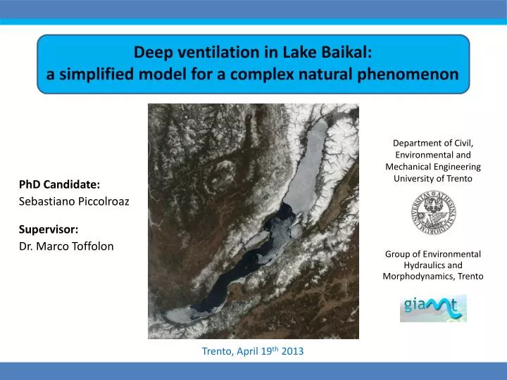
Deep ventilation in Lake Baikal: a simplified model for a complex natural phenomenon. Department of Civil, Environmental and Mechanical Engineering University of Trento. Group of Environmental Hydraulics and Morphodynamics, Trento. Trento, April 19 th 2013. Outline. Outline.

E N D
Deep ventilation in Lake Baikal: a simplified model for a complex natural phenomenon Department of Civil, Environmental and Mechanical Engineering University of Trento Group of Environmental Hydraulics and Morphodynamics, Trento Trento, April 19th 2013
Outline Outline Part 1 - A plunge into the abyss of the world's deepest lake • Lake Baikal and deep ventilation • A simplified 1D model • Calibration, validation, sensitivity analysis and main results • Climate change scenarios Part 2 – Back to the surface • A simple lumped model to convert Ta into surface Tw Conclusions
Part 1 A plunge into the abyss of the world's deepest lake
Lake Baikal Lake Baikal - Siberia (Озеро Байкал - Сибирь) The lake of records The oldest, deepest and most voluminous lake in the world
Lake Baikal Lake Baikal in numbers Lake Baikal formed in an ancient rift valley tectonic origin Divided into 3 sub-basins: South Basin Central Basin North Basin • Main characteristics: • Volume: 23 600 km3 Surface area: 31 700 km2 Length: 636 km Max. width: 79 km Max .depth: 1 642 m Ave. Depth: 744 m Shore Length: 2 100 km Surf. Elevation: 455.5 m Age: 25 million years Inflow rivers: 300 Outflow rivers: 1 (Angara River) World Heritage Site in 1996 1461 m
Lake Baikal Bathymetry An impressive bathymetry:maximum depth at 1642 m average depth at 744 m flat bottom steep sides Source: The INTAS Project 99-1669 Team. 2002. A new bathymetric map of Lake Baikal. Open-File Report on CD-Rom
Deep ventilation Deep ventilation The physical phenomenon • Phenomenon triggered by thermobaric instability [Weisset al., 1991]: • density depends on T and P (equation of state: Chen and Millero, 1976) • T of maximum density decreases with the depth (P=Patm Tρmax ≈ 4°C) ρparcel< ρlocal ehc 1 bar 10 m water hc strong weak external forcing ρparcel > ρlocal depth 2000 m Density ρ [kg m-3] ew<ehc NO DEEP DOWNWELLING ew>ehc DEEP DOWNWELLING depth 1000 m http://www.engineeringtoolbox.com depth 250 m ew ehc ew Temperature T [°C]
Deep ventilation A simplified sketch • The main effects: • deep water renewal • a permanent, even if weak, stratified temperature profile • high oxygen concentration up to the bottom deep ventilation at the shore wind sinking volume of water Presence of aquatic life down to huge depths
Deep ventilation The state of the art • Observations and data analysis: Weiss et al., 1991; Shimaraev et al., 1993; Hohmann et al., 1997; Peeters et al., 1997, 2000; Ravens et al., 2000; Wüest et al., 2000, 2005; Schmid et al., 2008; Shimaraev et al., 2009, 2011a,b, 2012 • Downwelling periods (May – June, December – January) • Downwelling temperature (3 ÷ 3.3 °C) • Downwelling volumes estimations (10 ÷ 100 km3 per year) • Numerical simulations: Akitomo, 1995; Walker and Watts, 1995; Killworth et al., 1996; Tsvetova, 1999; Peeters et al., 2000; Botte and Kay, 2002; Lawrence et al., 2002 • 2D or 3D numerical models • Simplified geometries or partial domains • Main aim: understand the phenomenon (triggering factors/conditions) Putin turns submariner at Lake Baikal Field measurement campaign (photo credit: C. Tsimitri) MIR: Deep Submergence Vehicle Walker and Watts, 1995
A simplified 1D numerical model A simplified 1D model The aims • simple way to represent the phenomenon (at the basin scale) • just a few input data required (according to the available measurements) • suitable to predict long-term dynamics (i.e. climate change scenarios) The site • South Basin of Lake Baikal The input data • surface water temperature (measurements + reanalysis) • wind speed and duration (observations + reanalysis) • Courtesy of Prof. A. Wüest and his research team (EAWAG) • ERA-40 reanalysis dataset, thanks to Clotilde Dubois and Samuel Somot (Meteo France) South Basin • Rzheplinsky and Sorokina, 1977 • ERA-40 reanalysis dataset, thanks to Clotilde Dubois and Samuel Somot (Meteo France)
A simplified 1D numerical model The model in three parts wind simplified downwelling algorithm(wind energy input vs energy required to reach hc) downwelling T profile Required energy → Available energy (downwelling volume) → Wind - based parameterization: ehc ehc Compensation depth - hc ξ and η: main calibration parameters of the model ew<ehc NO DEEP DOWNWELLING ew>ehc DEEP DOWNWELLING (mainly dependent on the geometry) ehc
A simplified 1D numerical model ρ The model in three parts Lagrangian vertical stabilization algorithm(re-arrange unstable regions, move the sinking volume) ρ °C • re-sorting starting form the pair of sub-volumes showing the higher instability • the mixing exchanges are accounted for at every switch Tρmax z where is the generic tracer and the mixing coeff. z Stable stable unstable Unstable
A simplified 1D numerical model The model in three parts vertical diffusion equation solver with source (reaction) terms (for temperature, oxygen and other solutes) DO °C • the diffusion equation is solved for any tracer • given the BC at the surface • and R along the water column. C Tρmax higher sat. conc. cooling flux oxygen consumption geothermal heat flux z flux z source oxygen consumption geothermal heat flux
A simplified 1D numerical model … it is a matter of feedback • Lacustrine systems are regulated by a complex network of feedback loops, controlled by the external forcing Self-consistent procedure to dynamically reconstruct Dz
Calibration Calibration Calibration procedure (ξ,η, cmix andDz,r) Medium term simulations during the second half of the 20th century: • comparison of simulated temperature and oxygenprofiles with measured data • formation of the CFC profile (1988-1996) unambiguous tracer: non-reactive, high chemical stability [e.g. England, 2001] Objective: numerically reproduce particular conditions of the lake during a specific historical period (1980s- 1990s). Available data: reanalysisdataset the reprocessing of past climate observations combining together data assimilation techniques and numerical modeling (GCMs) ERA-40 datasets: wind speed (W) and air temperature (Ta) every 6 hours from1958 to 2002 Thanks to S. Somot and C. Dubois (Meteo France)
Calibration Reanalysis data: limitations • reanalysis horizontal resolution is too coarse (∼ 100 km x 100 km) for the purpose of many practical applications (mismatch of spatial scales) • reanalysis data are often affected by inconsistencies due to the lack of fundamental feedback between the numerous natural processes • air temperature is available, but the model requires surface water temperature Post-processing (downscaling) is necessary
Calibration Statistical downscaling Transfer function approach: establishes a relationship between the cumulative distribution functions (CDFs) of observed local climate variables (predictands) and the CDFs of large-scale GCMs outputs (predictors) Quantile – mapping method [Panofsky and Brier, 1968]: assumption xr = generic climatic variable of re-analysis (W, Ta) Xr,adj = generic climatic variable adjusted CDFr = cumulative distribution function of re-analysis data CDFo = cumulative distribution function of observations [e.g. Minville et al.,2008; Diaz-Nieto and Wilby, 2005; Hay et al., 2000] • Drawbacks: • it does not include information of future climate patterns • it is stationary in the variance and skew of the distribution, and only the mean changes • it is not indicated to be applied for climate change analysis
Calibration Quantile-mapping approach From reanalysis (large scale) to observations (local scale) Wind: seasonal CDFs Temperature: daily CDFs Wr,adj Tw,adj Wr Ta,r
Calibration Temperature profiles 15th of February 15th of September
Calibration CFC and dissolved oxygen profiles Mean annual
Sensitivity analysis Sensitivity analysis • Results: • an evident deviation from measurements and calibrated solution • suggesting that a proper calibration has been achieved • no dramatic changes are observed in the behavior of the limnic system • indicating the suitability and robustness of the fundamental algorithms Sensitivity analysis Aimed at evaluating the robustness of the calibration and the role played by each of the main parameters of the model. Procedure: a new set of 40-year simulations, changing ξ,η and cmix (one by one) within the interval of ± 50% of the calibrated value.
Validation Validation Validation procedure Limited amount of available information a classical validation of this model with an independent set of data is not possible adjustment phase ∼ 50 – 100 years asymptotic equilibrium T ∼ 3.37°C • Indirect validation: long-term simulation, starting from arbitrarily set initial conditions and verifying the achievement of proper equilibrium profiles of the main variables. • Initial conditions:isothermal (T=3.98°C) and anoxic profiles (DO=0 mgO2 l-1) • Boundary conditions: a series of 1000 years randomly generated from the ERA-40 reanalysis dataset Same external forcing as those of current conditions numerical results are expected to converge toward the actual observed conditions, after an adjustment phase depending on the IC.
Validation Temperature and dissolved oxygen profiles 15th of February Mean annual
Main results Main results Characterization of seasonal dynamics • cycle of temperature • thickness of the epilimnion • diffusivity profile • N2, S2 and Ri profiles In-depth analysis of deep ventilation • timing of deep ventilation • vertical distribution of downwellings • main downwelling properties: and • energy demand vs.
Main results Seasonal cycle of temperature (mean year) RMSE ∼ 0.07°C MAE ∼ 0.03°C MaxAE ∼ 0.78°C Simulation (1000-year simulation, mean year) Measurements (data courtesy of Prof. A. Wüest, unpublished data) Map of residuals (modeled - measured temperature profiles).
Main results Downwelling propertiesmean annual sinking volume ( ) and temperature ( ) Warm season: smaller and colder events Cold season: larger and warmer events Present model: statistics based on the 1000-year simulation results (long dataset) events beneath 1300 m depth Literature estimates: measurements collected near the bottom short observational periods (from a few years to a decade) significant variability between the single authors (depending on analyzed events) is probably underestimated[Wüest et al., 2005; Schmid et al., 2008]
Main results Downwelling propertiesrelationship between and the specific energy required to reach hc Warm season: smaller and colder events Cold season: larger and warmer events Wind is stronger during the cold season (Oct-Dec) is larger during this period … Wind-speed parameterization: ec is higherin winter … and is higher. One would expect colder in winter than in summer Is this a contradictory result? Seasonality of ec due to the typical thermal structure of the epilimnion
Climate change Climate change The aim • investigate the future response of the limnic system to climate change • estimate the possible impact on deep ventilation The scenarios Constructed on the basis of the outputs from GCMs forced with different greenhouse gases (GHG) concentration projections (IPCC 2007) CMIP5 datasets: wind speed (W) and air temperature (Ta) every 3 hours for the 3 different scenarios (rcp2.6, rcp 4.5 and rcp8.5) and the following periods 1960-2005, 2026-2046 and 2081-2101. Thanks to S. Somot and C. Dubois (Meteo France)
Climate change CMIP5 data: limitations • mismatch of spatial scales, simplification of natural phenomena, no information regarding Tw(as for re-analysis data) • due to their different derivation, CMIP5 data cannot be considered as the prosecution of the re-analysis series downscaling compatibility bias in theascending branch Bias during the whole year Coarse resolution, global scale climate patterns
Climate change Data processing: downscaling Wind speed (W): a novel procedure has been developed, based on the quantile-mapping approach, but also accounts for potentialmodifications in both intensity and seasonality of wind speed. Air temperature (Ta): a simple lumped model to convertTa into surface Tw to assess the possible impact on lake temperature (ΔTw) quantile-mapping approach, including ΔTw (delta method) ΔTw Conversion… Air 2 Water Tw,fut ΔTw Ta,r Tw,adj
Climate change Temperature profiles 15th of February 15th of September
Climate change Oxygen profiles The main changes are expected for the RCP8.5 scenario: evident enhancement of deep water renewal (larger and colder downwelling volumes, strong oxygenation) the major impact is expected from modifications of the wind forcing (intensity and seasonality) Mean annual
Part 2 Back to the surface
Conversion Ta→Tw 1/2 Tool: a simplified, physically-based multi-parametric model that solves the heat exchanges between lake and air Air2Water Air2Water The model A simple lumped model to convert air temperature (Ta) into surface water temperature (Tw) of lakes model Main forcing factor: air temperature Ta Ta Tw physical parameters Main result: surface water temperature Tw The key equation Heat budget in the well-mixed surface layer
Air2Water The heat budget A simplified parameterization of the net heat exchange seasonal forcing (hp. sinusoidal) residual effect of Tw “gradient” with atmosphere residual 1 effect of time-dependent stratification: dimensionless depth of the surface well-mixed layer (Tr is the deep temperature, for dimictic lakes =4°C) • Different versions of the model: • 8-parameter (pi, i=1..8) • 6-parameter (pi, i=1..6) simplified inverse stratification (winter) • 4-parameter (pi, i=3..6) seasonal forcing included in the other periodic terms (p4, p5)
Air2Water An application to Lake Superior (4 par. model) Selection of parameters based on Nash efficiencyindex (108 Monte Carlo model realizations with uniform random sampling) calibration validation T air meas. T water model 4 par. model 8 par meas.
Air2Water … using satellite data T air meas. T water model 4 par. model 8 par meas. (data: Great Lakes Environmental Research Laboratory, NOAA National Oceanic and Atmospheric Administration) • The model has been applied to other lakesBaikal (Russia), Great Lakes (USA-Canada), Garda (Italy) and Mara (Canada) • The model is suitable to reproduce the evolution of Tw at long time scales seasonal, annual, inter-annual hysteresis cycle and inter-annual fluctuations
a simplified numerical model has been developed to simulate deep ventilation andanalyze downwelling dynamics in profound lakes (Lake Baikal) Conclusions Conclusions • Main results: • a simplified numerical model has been developed to simulate deep ventilation in profound lakes (Lake Baikal) • the model allows for a suitable description of seasonal lake dynamics and a proper evaluation ofdownwelling features (e.g. and ) • some preliminary evidence about the existence of significant feedback loops among the different physical processes has been found (e.g. ecvs ) • thanks to its simple structure (low computational cost) and suitable parameterization (necessary to investigate evolving systems) such a model is appropriate to predict long-term dynamics (i.e. climate change scenarios) • a novel downscaling procedure and a simple physically-based model to convert air temperature into surface water temperature have been devised, which are suitable to be applied in climate change studies
Further activities: • further research is expected to explore the coupling of physical and biological processes (e.g. plankton dynamics) • further research is needed to better understand the complex network of interactions between the numerous physical processes that take place in the lake • the model could be used to investigate the convective dynamics in the other very deep lakes in the world (e.g. Lake Tanganyika, Crater Lake) and possibly also is some deep alpine lakes (e.g.LakeTahoe, Lake Como, Lake Geneva, Lake Garda) • Air2Water is expected to be applied to lakes having different characteristic (e.g. geometry, climate, mixing regime) in order to assess the possibleresponse of the lake to differentclimateconditions. Diatoms viewed through the microscope. Image by Dr. G.T. Taylor Light micrograph of diatom Amphorotia hispida discovered in Lake Baikal, Lake Garda (Italy)
Thank you sebastiano.piccolroaz@ing.unitn.it Thank you Mysterious ice circles in the southern basin of Lake Baikal (Nasa Earth Observatory, April 25, 2009; Balkhanov et al., TP 2010)