Download
1 / 22
220 likes | 235 Views
New Computational Insights from Quantum Optics. Scott Aaronson Based on joint work with Alex Arkhipov. The Extended Church-Turing Thesis (ECT) Everything feasibly computable in the physical world is feasibly computable by a (probabilistic) Turing machine.

E N D
New Computational Insights from Quantum Optics Scott Aaronson Based on joint work with Alex Arkhipov
The Extended Church-Turing Thesis (ECT) Everything feasibly computable in the physical world is feasibly computable by a (probabilistic) Turing machine But building a QC able to factor n>>15 is damn hard! Can’t CS “meet physics halfway” on this one?I.e., show computational hardness in more easily-accessible quantum systems? Also, factoring is a “special” problem
Our Starting Point All I can say is, the bosons got the harder job In P #P-complete [Valiant] BOSONS FERMIONS
So if n-boson amplitudes correspond to permanents… Can We Use Bosons to Calculate the Permanent? That sounds way too good to be true—it would let us solve NP-complete problems and more using QC! Explanation: Amplitudes aren’t directly observable. To get a reasonable estimate of Per(A), you might need to repeat the experiment exponentially many times
Basic Result: Suppose there were a polynomial-time classical randomized algorithm that took as input a description of a noninteracting-boson experiment, and that output a sample from the correct final distribution over n-boson states. Then P#P=BPPNP and the polynomial hierarchy collapses. Motivation: Compared to (say) Shor’s algorithm, we get “stronger” evidence that a “weaker” system can do interesting quantum computations
Crucial step we take: switching attention to sampling problems P#P SampBQP Permanent BQP PH SampP xy… BPPNP Factoring 3SAT BPP
Related Work Valiant 2001, Terhal-DiVincenzo 2002, “folklore”:A QC built of noninteracting fermions can be efficiently simulated by a classical computer Knill, Laflamme, Milburn 2001: Noninteracting bosons plus adaptive measurementsyield universal QC Jerrum-Sinclair-Vigoda 2001: Fast classical randomized algorithm to approximate Per(A) for nonnegative A A. 2011:Generalization of Gurvits’s algorithm that gives better approximation if A has repeated rows or columns
The Quantum Optics Model Classical counterpart: Galton’s Board, on display at the Boston Museum of Science Using only pegs and non-interacting balls, you probably can’t build a universal computer—but you can do some interesting computations, like generating the binomial distribution! A rudimentary subset of quantum computing, involving only non-interacting bosons, and not based on qubits
The Quantum Version Then we see strange things like the Hong-Ou-Mandel dip The two photons are now correlated, even though they never interacted! Let’s replace the balls by identical single photons, and the pegs by beamsplitters Explanation involves destructive interference of amplitudes:Final amplitude of non-collision is
Getting Formal The basis states have the form |S=|s1,…,sm, where si is the number of photons in the ith “mode” We’ll never create or destroy photons. So s1+…+sm=n is constant. U For us, m=poly(n) Initial state: |I=|1,…,1,0,……,0
You get to apply any mm unitary matrix U If n=1 (i.e., there’s only one photon, in a superposition over the m modes), U acts on that photon in the obvious way In general, there are ways to distribute n identical photons into m modes U induces an MM unitary (U) on the n-photon states as follows: Here US,T is an nn submatrix of U (possibly with repeated rows and columns), obtained by taking si copies of the ith row of U and tj copies of the jth column for all i,j
Beautiful Alternate Perspective The “state” of our computer, at any time, is a degree-n polynomial over the variables x=(x1,…,xm) (n<<m) Initial state: p(x) := x1xn We can apply any mm unitary transformation U to x, to obtain a new degree-n polynomial Then on “measuring,” we see the monomialwith probability
OK, so why is it hard to sample the distribution over photon numbers classically? Given any matrix ACnn, we can construct an mm unitary U (where m2n) as follows: Suppose we start with |I=|1,…,1,0,…,0 (one photon in each of the first n modes), apply U, and measure. Then the probability of observing |I again is
Claim 1: p is #P-complete to estimate (up to a constant factor) Idea: Valiant proved that the Permanent is #P-complete. Can use a classical reduction to go from a multiplicative approximation of |Per(A)|2 to Per(A) itself. Claim 2: Suppose we had a fast classical algorithm for boson sampling. Then we could estimate p in BPPNP Idea: Let M be our classical sampling algorithm, and let r be its randomness. Use approximate counting to estimate Conclusion: Suppose we had a fast classical algorithm for boson sampling. Then P#P=BPPNP.
The Elephant in the Room The previous result hinged on the difficulty of estimating a single, exponentially-small probabilityp—but what about noise and error? The “right” question: can a classical computer efficiently sample a distribution with 1/poly(n) variation distance from the boson distribution? Our Main Result: Suppose it can. Then there’s a BPPNP algorithm to estimate |Per(A)|2, with high probability over a Gaussian matrix
Our Main Conjecture Estimating |Per(A)|2, for most Gaussian matrices A, is a #P-hard problem If the conjecture holds, then even a noisy n-photon experiment could falsify the Extended Church Thesis, assuming P#PBPPNP! Most of our paper is devoted to giving evidence for this conjecture We can prove it if you replace “estimating” by “calculating,” or “most” by “all”
First step: understand the distribution of |Per(A)|2 for random A Conjecture: There exist constants C,D and >0 such that for all n and >0, Empirically true! Also, we can prove it with determinant in place of permanent
The Equivalence of Sampling and Searching[A., CSR 2011] [A.-Arkhipov] gave a “sampling problem” solvable using quantum optics that seems hard classically—but does that imply anything about more traditional problems? Recently, I found a way to convert any sampling problem into a search problem of “equivalent difficulty” Basic Idea: Given a distribution D, the search problem is to find a string x in the support of D with large Kolmogorov complexity
Using Quantum Optics to Prove that the Permanent is #P-Hard[A., Proc. Roy. Soc. 2011] Valiant famously showed that the permanent is #P-hard—but his proof required strange, custom-made gadgets • We gave a new, more transparent proof by combining three facts: • n-photon amplitudes correspond to nn permanents • (2) Postselected quantum optics can simulate universal quantum computation [Knill-Laflamme-Milburn 2001] • (3) Quantum computations can encode #P-hard quantities in their amplitudes
Experimental Issues • Basically, we’re asking for the n-photon generalization of the Hong-Ou-Mandel dip, where n = big as possible • Our results suggest that such a generalized HOM dip would be evidence against the Extended Church-Turing Thesis Physicists: “Sounds hard! But not as hard as full QC” Remark: If n is too large, a classical computer couldn’t even verify the answers! Not a problem yet though… Several experimental groups (Imperial College, U. of Queensland) are currently working to do our experiment with 3 photons. Largest challenge they face: reliable single-photon sources
Summary • Thinking about quantum optics led to: • A new experimental quantum computing proposal • New evidence that QCs are hard to simulate classically • A new classical randomized algorithm for estimating permanents • A new proof of Valiant’s result that the permanent is #P-hard • (Indirectly) A new connection between sampling and searching
Open Problems Prove our main conjecture: that Per(A) is #P-hard to approximate for a matrix A of i.i.d. Gaussians ($1,000)! Can our model solve classically-intractable decision problems? Fault-tolerance in the quantum optics model? • Find more ways for quantum complexity theory to “meet the experimentalists halfway” • Bremner, Jozsa, Shepherd 2011: QC with commuting Hamiltonians can sample hard distributions