Download
1 / 41
410 likes | 502 Views
Intervention models. Something’s happened around t = 200. The first example. Seems like a series that is generally stationary, but shifts level around t = 200. Look separately at the parts before and after the level shift.

E N D
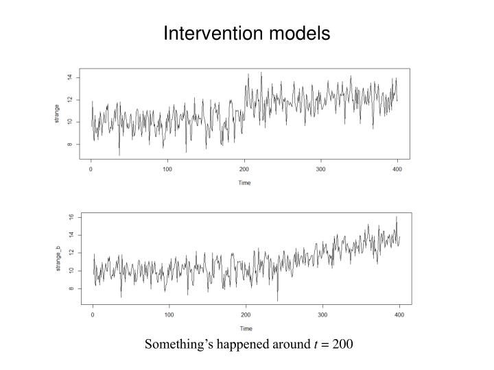
Intervention models Something’s happened around t = 200
The first example Seems like a series that is generally stationary, but shifts level around t = 200. Look separately at the parts before and after the level shift. There are in total 400 time-points. Select the first 190 and the last 190
First 190 values Could be an AR(1) or an MA(1) or an ARMA(1,1). Quite clearly stationary!
Last 190 values Points more towards an ARMA(1,1)
The change in level would most probably be modelled using a step function A complete intervention model for the times series can therefore be since there seems to be a permanent immediate constant change in level at t = 200 How can this model be fitted using R?
strange.model <-arimax(strange,order=c(1,0,1), xtransf=data.frame(step200=1*(seq(strange)>=200)), transfer=list(c(0,0))) The arimax command works like the arima command, but allows inclusion of covariates. The argument xtransf is followed by a data frame in which each column correspond to a covariate time series (same number of observations as Yt ). Here this data frame is constructed with the command 1*(seq(strange)>=200) The command seq(strange) returns the indices of the vector strange The command seq(strange)>=200 returns a vector (with the same length as strange in which a term is FALSE if the corresponding index of strange is less than 200 and TRUE otherwise. Finally, the multiplication with 1 transforms FALSE into 0 and TRUE into 1 and the variable in the data frame is also given the name step200 (for convenience) Hence, the resulting column is a step function of the kind we want.
The argument transfer is followed by a list comprising one two-dimensional vector for each covariate specified by xtransf Here we have the argument list(c(0,0)) implying that the covariate shall be included as it stands (no lagging, no filtering). Note that the argument must always be followed by a list (even if there is only one covariate). Giving an argument c(r,s) where both r and s are > 0 will enter the term into the model. Since we have specified c(0,0) the term included will be
print(strange.model) Series: strange ARIMA(1,0,1) with non-zero mean Coefficients: ar1 ma1 intercept step200-MA0 0.9824 -1.0000 10.0026 1.9958 s.e. 0.0111 0.0064 0.0350 0.0606 sigma^2 estimated as 0.9826: log likelihood=-564.82 AIC=1137.64 AICc=1137.79 BIC=1157.6 Thus, the estimated model is
tsdiag(strange.model) Seems to be some autocorrelation left in the residuals. Try an ARMA(1,2)
strange.model2 <-arimax(strange,order=c(1,0,2), xtransf=data.frame(step200=1*(seq(strange)>=200)), transfer=list(c(0,0))) • print(strange.model2) • Series: strange • ARIMA(1,0,2) with non-zero mean • Coefficients: • ar1 ma1 ma2 intercept step200-MA0 • 0.9730 -0.7781 -0.2219 10.0012 1.9972 • s.e. 0.0133 0.0525 0.0521 0.0317 0.0557 • sigma^2 estimated as 0.9406: log likelihood=-556.28 • AIC=1122.56 AICc=1122.77 BIC=1146.5 Coefficients seem to be significantly different from zero (divided by s.e. and compare with 2) Log-likelihood slightly higher.
tsdiag(strange.model2) Clear improvement!
plot(y=strange,x=seq(strange),type="l",xlab="Time") lines(y=fitted(strange.model),x=seq(strange),col="blue", lwd=2) lines(y=fitted(strange.model2),x=seq(strange),col="red", lwd=1) legend("bottomright",legend=c("original","model1","model2"),col=c("black","blue","red"),lty=1,lwd=c(1,2,1)) Model 2 (ARMA(1,2) is less smooth, but may follow the correlation structure better. However, this cannot be clearly seen from the plot.
The second example Seems like a series that is from the beginning stationary, but gets a linear drift (upward trend) around t = 200. Look at the part before . There are in total 400 time-points. Select the first 200.
First 200 values Looks (again) like an ARMA(1,1)
eacf(strange[1:200]) AR/MA 0 1 2 3 4 5 6 7 8 9 10 11 12 13 0 x o o o o o o o o o o o o o 1 o o o o o o o o o o o o o o 2 x o o o o o o o o o o o o o 3 x x x o o o o o o o o o o o 4 o x x o o o o o o o o o o o 5 o x x o o o o o o o o o o o 6 x x o o o o o o o o o o o o 7 x x o o o o o o o o o o o o
The drift in level could be modelled using a linearly increasing step function A complete intervention model for the times series can therefore be
The term will be problematic to estimate. However, the following holds Hence, create a covariate that is 0 until t = 200 and then 1, 2, …, 200 and use it with transfer=list(c(0,0)) Alternatively, and more efficient is to include this variable as an ordinary explanatory variable (a regression predictor), using the argument xreg
strange_b.model <-arimax(strange_b,order=c(1,0,1), xreg=data.frame(x=c(rep(0,200),1:200))) print(strange_b.model) Call: arimax(x = strange_b, order = c(1, 0, 1), xreg = data.frame(x = c(rep(0, 200), 1:200))) Coefficients: ar1 ma1 intercept x 0.1219 0.0382 9.9993 0.0192 s.e. 0.3783 0.3827 0.0744 0.0009 sigma^2 estimated as 0.9884: log likelihood = -565.25, aic = 1138.5 Note! This can also be seen as a simple linear regression model with ARMA(1,1) error terms.
tsdiag(strange_b.model) Satisfactory!
Transfer-function models Consider the data set boardings referred to in Exercise 11.16 data(boardings) summary(boardings) log.boardings log.price Min. :12.40 Min. :4.649 1st Qu.:12.49 1st Qu.:4.973 Median :12.53 Median :5.038 Mean :12.53 Mean :5.104 3rd Qu.:12.57 3rd Qu.:5.241 Max. :12.70 Max. :5.684 Two time-series, both with log-transformed values
plot.ts(boardings) Could the price affect the boardings?
The cross-correlation function …measures the degree of linear dependence between the two series
Sample cross-correlation function With R: ccf For the boardings data set, we can try to calculate the cross-correlation function between the two series
ccf(boardings[,1],boardings[,2],main=”boardings & price”, ylab=”CCF”) Typical look when at least one of the times series is non-stationary
Take first-order regular differences diff_boardings<-diff(boardings[,1]) diff_price<-diff(boardings[,2]) ccf(diff_boardings,diff_price,ylab=”CCF”) Still not satisfactory. Since we have monthly data, we should possibly try first-order seasonal differences as well.
diffs_boardings<-diff(diff_boardings,12) diffs_price<-diff(diff_price,12) ccf(diffs_boardings,diffs_price,ylab=”CCF”)) Better, but how do we interpret this plot? The two significant spikes for negative lags says that the difference in price depends on the difference in boardings some months earlier. The significant spike at lag 6 says that the difference in boardings depends on the difference in price some months earlier. What explains what?
A problem: Since both series would show autocorrelations, these are unevitably part of the cross-correlations we are estimating (cf. auto-correlation and partial auto-correlation). To solve this we need to “remove” the autocorrelation in the two series before we investigate the cross-correlation. We should estimate cross-correlations between residual series from modelling with ARMA-models This procedure is known as pre-whitening Normal procedure: Find a suitable ARMA model for the (differenced) series that is assumed to constitute the covariate series. Fit this model to both series Investigate the cross-correlations between the residual series.
Could be an ARMA(1,1,1,0)12 or an ARMA(1,1,1,1)12
model1=arima(diffs_price,order=c(1,0,1),seasonal=list(order=c(1,0,0),lag=12))model1=arima(diffs_price,order=c(1,0,1),seasonal=list(order=c(1,0,0),lag=12)) tsdiag(model1) Could do!
model2=arima(diffs_price,order=c(1,0,1),seasonal=list(order=c(1,0,1),lag=12))model2=arima(diffs_price,order=c(1,0,1),seasonal=list(order=c(1,0,1),lag=12)) tsdiag(model2) Better! Ljung-Box was not possible to do here!
Applying the last model to the differenced boardings series model21=arima(diffs_boardings,order=c(1,0,1),seasonal=list(order=c(1,0,1),lag=12)) ccf(residuals(model2),residuals(model21),ylab="CCF") Well, not that much cross-correlation left…
THE TSA package provide the command prewhiten with which prewhitening is made and the resulting CCF is plotted. The default set-up is that an AR model is fit to the covariate series (the first series specified. The AR model that minimizes AIC is chosen The model can however be specified.
prewhiten(diffs_price,diffs_boardings,x.model=model2, ylab="CCF") Should be the same as the manually developed CCF earlier
With the default settings pw=prewhiten(diffs_price,diffs_boardings,ylab="CCF") Picture is clearer? No significant cross-correlations left What AR model has been used?
print(pw) $ccf Autocorrelations of series ‘X’, by lag -1.0833 -1.0000 -0.9167 -0.8333 -0.7500 -0.6667 -0.5833 -0.5000 -0.4167 -0.3333 -0.2500 -0.1667 -0.0833 0.0000 0.0833 0.1667 0.131 0.057 -0.053 -0.167 -0.034 0.120 0.228 -0.129 -0.181 0.009 0.164 0.100 0.098 0.031 -0.065 0.019 0.2500 0.3333 0.4167 0.5000 0.5833 0.6667 0.7500 0.8333 0.9167 1.0000 1.0833 -0.023 -0.078 -0.349 0.027 -0.155 -0.225 0.041 -0.027 -0.167 -0.097 0.200 $model Call: ar.ols(x = x) Coefficients: 1 2 3 4 5 6 7 8 9 10 -0.2145 0.0361 -0.1226 -0.4786 -0.1827 0.1392 -0.0133 0.1616 -0.1462 0.1395 Intercept: 0.002233 (0.00302) Order selected 10 sigma^2 estimated as 0.0004016
Check with a scatter plot Reasonable that there is no significant cross-correlation
Another example Observations of the input gas rate to a gas furnace and the percentage of carbon dioxide (CO2) in the output from the same furnace stationary? stationary?
gasrate series Not that far from stationary. In that case an AR(2) would be the first choice. However, we also try first-order regular differences gasrate_diff< diff(gasrate)
CO2 series Stationary. AR(2) ?