Download
1 / 24
240 likes | 257 Views
HT Lecture on Nonlinear beam dynamics (I). HT Lecture on Nonlinear beam dynamics (II). Hamiltonian of the nonlinear betatron motion Resonance driving terms Tracking Dynamic Aperture and Frequency Map Analysis Spectral Lines and resonances Nonlinear beam dynamics experiments at Diamond.

E N D
HT Lecture on Nonlinear beam dynamics (I) HT Lecture on Nonlinear beam dynamics (II) Hamiltonian of the nonlinear betatron motion Resonance driving terms Tracking Dynamic Aperture and Frequency Map Analysis Spectral Lines and resonances Nonlinear beam dynamics experiments at Diamond Motivations: nonlinear magnetic multipoles Phenomenology of nonlinear motion Simplified treatment of resonances (stopband concept) Hamiltonian of the nonlinear betatron motion
The Hamiltonian for the nonlinear betatron motion is given by Hamiltonian of nonlinear betatron motion We define H0 the linear part (dependent only on dipoles and normal quadrupoles) and V the nonlinear part dependent on the nonlinear magnetic multipoles Normal multipoles skew multipoles
We define a canonical transformation that reduces the linear part of the Hamiltonian to a rotation canonical transformation Normalisation of the linear part of the Hamiltonian with generating function In detail linear Courant-Snyder invariant This transformation reduces ellipses in phase space to circles and the motion to a rotation along these circles, for linear systems
The new Hamiltonian reads Resonance driving terms (I) The hjklmp are called resonance driving terms since they generate angle dependent terms in the Hamiltonian that are responsible for the resonant motion of the particles (i.e. motion on a chain of islands or on a separatrix). On the islands the betatron tuned satisfy a resonant condition of the type NQx + MQy = p resonance (N, M) N = j – k and M = l – m Terms of the type hjjkkp produce detuning with amplitude to the lowest order in the multipolar gradient, but they can interfere with other terms in the Hamiltonian to create resonances (perturbative theory of betatron motion) Without angle dependent term the motion will be just an amplitude dependent rotation
The dynamics with angle dependent terms exhibits fixed points, island e.g. for the (4,0) resonance The dynamics with only detuning terms is an amplitude dependent rotation Non resonant and single resonance Hamiltonian
The resonant driving terms are integrals over the whole length of the accelerator of functions which depend on the s-location of the multipolar magnetic elements Resonance driving terms (II) The solution for the stable betatron motion can be written as a quasi periodic signal to first order in the multipoles strengths with Each resonance driving term hjklmp contributes to the Fourier coefficient of a well precise spectral line
Let us consider the driving terms generated by a normal sextupole. In the general definition of driving term Resonance driving terms from sextupoles We substitute the function that give the azimuthal distribution of the normal sextupoles along the ring generate the following resonant driving terms (see Guignard, Bengtsson) from V30 j+k = 3; l+m =0 exciting the resonances (3, 0) (1, 0) (1, 2) (1, –2)
Consider a linear lattice with a single sextupole kick. The resonance driving terms h3000 exciting the third order resonance (3,0) generates the frequency Example: third order resonance with a sextupole Far from the resonant values Qx = p/3 e.g. Qx = 0.31 – 2Qx = –0.62 0.38 the lines Qx and -2Qx are well separated Approaching the resonant value Qx = 1/3 Qx = 0.33 – 2Qx = –0.66 0.34 the tune spectral line (Qx) and the h3000 spectral line (-2Qx) coalesce
In an analogous way we can see that the normal octupoles in the circular ring Resonance driving terms from octupoles generate the following resonant driving terms (see Guignard, Bengtsson) from V40 j+k = 4; l+m =0 from V22 j+k = 2; l+m =2 from V04 j+k = 0; l+m =4 exciting the resonances (4, 0) (2, 0) (2, 2) (2, –2) (0, 2) (0,4)
From the analysis of the Fourier expansion of the driving term we can infer simple rules to compensate the effect of strongly excited nonlinearities The aim is to reduce the driving term Resonance compensation We have to find suitable distribution of nonlinear magnetic elements along the ring, i.e. suitable functions Vm,n(s) that reduce or cancel those driving terms which are stronger in the uncorrected machine. Typically two equal sextupoles at 60 degree phase advance apart compensate each other, in the (3,0) resonance driving term (and p=0 which is the strongest term) In an analogous way two equal octupoles at 45 degree phase advance apart compensate each other in the (4,0) driving terms However their effect on all the other resonances has to be assessed!
Let us consider the nonlinear Hill’s equation for the case of a linear lattice where a single sextupole kick is added Can a sextupole excite a 4-th order resonance? (I) Let us use a perturbative procedure and try to solve this equation by successive approximations. The perturbation parameter is proportional to the sextupole strength k2. We look for a solution of the type: Substituting, ordering the contributions with the same perturbative order we have order zero: 0 first order: 1 second order: 2
At each step we are using functions already calculated at the previous steps Linear solution Can a sextupole excite a 4-th order resonance? (II) Term generated by the 3rd order resonance; linear with k2 (first order) Terms generated by the 4th order and 2nd order resonance; quadratic with k2 (second order) The series obtained from the successive approximation are in general divergent, however the first term of the series, judiciously chosen, offer a good approximation of the nonlinear betatron motion
The equations can be solved numerically. The phase space plots of the motion of a charged particle in a lattice with a single thin sextupole are given by Q = 1/3 +0.005 smaller scales in plot Tiny dynamic aperture Q = 1/4 +0.005 Can a sextupole excite a 4-th order resonance? (III) Q = 1/5 +0.005 Q = 1/6 +0.005 Tracking particles close to the resonant tune value, starting at the same tune distance from the resonance, show that a sextupole can excite all higher order resonances. The islands width is smaller for higher orders, i.e. the corresponding resonances are weaker
Most accelerator codes have tracking capabilities: MAD, MADX, Tracy-II, elegant, AT, BETA, transport, … Typically one defines a set of initial coordinates for a particle to be tracked for a given number of turns. The tracking program “pushes” the particle through the magnetic elements. Each magnetic element transforms the initial coordinates according to a given integration rule which depends on the program used, e.g. transport (in MAD) Tracking (I) Linear map Nonlinear map up to third order as a truncated Taylor series
A Hamiltonian system is symplectic, i.e. the map which defines the evolution is symplectic (volumes of phase space are preserved by the symplectic map) M is symplectic transformation Tracking (II) non symplectic Symplectic integrator If the integrator is not symplectic one may found artificial damping or excitation effect The well-known Runge-Kutta integrators are not symplectic. Likewise the truncated Taylor map is not symplectic. They are good for transfer line but they should not be used for circular machine in long term tracking analysis Elements described by thin lens kicks and drifts are always symplectic: long elements are usually sliced in many sections.
The Frequency Map Analysis is a technique introduced in Accelerator Physics form Celestial Mechanics (Laskar). It allows the identification of dangerous non linear resonances during design and operation. Strongly excited resonances can destroy the Dynamic Aperture. Frequency Map Analysis To each point in the (x, y) aperture there corresponds a point in the (Qx, Qy) plane The colour code gives a measure of the stability of the particle (blu = stable; red = unstable) The indicator for the stability is given by the variation of the betatron tune during the evolution: i.e. tracking N turns we compute the tune from the first N/2 and the second N/2
Frequency Map Measurement (I) The measurement of the Frequency Map requires a set of two independent kickers to excite betatron oscillations in the horizontal and vertical planes of motion; The Beam Position Monitors (BPMs) must have turn-by-turn capabilities (at least one !) in order to be able to measure the tunes from the induced betatron oscillations; The betatron tune is generally the frequency corresponding to the maximum amplitude in the spectrum;
Frequency Map Measurement (II) A example of betatron oscillations recorded after a kick in the vertical plane at diamond. 256 turns are recored: the time signals of many kicks is superimposed to check the reproducibility of the kick and of the oscillations, small variation in the betatron tunes are detected (2e-4).
FM measurement at the Advanced Light Source Advanced Light Source Energy = 1.5 – 1. 9 GeV Circumference 198.6 m Two single turn pinger H and V (600 ns) Turn by Turn BPMs 40 electron bunches – 10 mA Used LOCO to set the linear lattice and restore super-periodicity (12–fold) ALS measured ALS model 4Qx + Qz 3Qx + 2Qz Very good comparison machine – model !
Dynamic Aperture: SOLEIL’s example SOLEIL bare lattice at zero chromaticity Black–model; Blue–loss rate; Red unstable Black–model; Colours measured Tracking includes Systematic multipole errors Dipole: up to 14-poles Quadrupoles: up to 28-poles Sextupoles: up to 54-poles Correctors (steerers): up to 22-poles Secondary coils in sext. strong 10-pole term From magnetic measurements: Dipole: fringe field, gradient error, edge tilt errors Coupling errors (random rotation of quadrupoles) No quadrupole fringe fields
Using a kicker and two BPMs with a known phase advance we can reconstruct the orbit in phase space. Typically if the BPMs are at 90 degrees with the same one can recover x and x’ and plot the phase space Phase space orbit analysis Diamond horizontal phase space close to the 5th order resonance (2000 turns) The damping in amplitude is not simply due to radiative damping but mainly to the fact that the centre of charge of the bunch is undergoing filamentation in phase space (decoherence)
All Diamond BPMs have turn-by-turn capabilities • excite the beam diagonally • measure tbt data at all BPMs • colour plots of the FFT H Frequency spectrum measured at all BPMs at Diamond BPM number QX = 0.22 H tune in H Qy = 0.36 V tune in V V All the other important lines are linear combination of the tunes Qx and Qy BPM number m Qx + n Qy frequency / revolution frequency
Detuning with amplitude and next to leading frequencies from turn-by-turn data FFT as a function of the kicker strength Qx seen in the V plane: (1,1) resonance Qy seen in the H plane: (1,1) resonance 2Qx seen in the H plane: (3,0) resonance 2Qy seen in the H plane: (1,2) resonance The information in the spectral lines can be used to compensate the resonant driving terms and improve the dynamic aperture of the ring
E. Wilson, CAS Lectures 95-06 and 85-19 E. Wilson, Introduction to Particle Accelerators G. Guignard, CERN 76-06 and CERN 78-11 J. Bengtsson, Nonlinear Transverse Dynamics in Storage Rings, CERN 88-05 J. Laskar et al., The measure of chaos by numerical analysis of the fundamental frequncies, Physica D65, 253, (1992). Bibliography