Download
1 / 16
210 likes | 980 Views
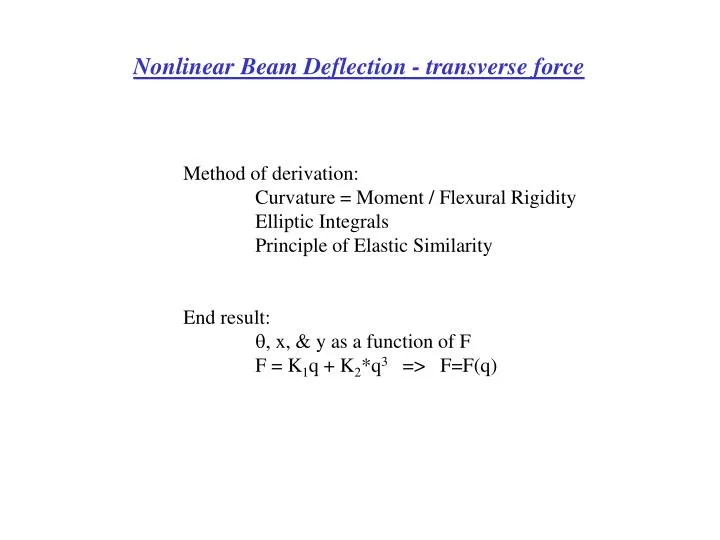
Nonlinear Beam Deflection - transverse force. Method of derivation: Curvature = Moment / Flexural Rigidity Elliptic Integrals Principle of Elastic Similarity End result: q, x, & y as a function of F F = K 1 q + K 2 *q 3 => F=F(q). y. EI. L. x. ds. dy. F 0. d. Y. dx. 1.

E N D
Nonlinear Beam Deflection - transverse force Method of derivation: Curvature = Moment / Flexural Rigidity Elliptic Integrals Principle of Elastic Similarity End result: q, x, & y as a function of F F = K1q + K2*q3 => F=F(q)
y EI L x ds dy F0 d Y dx 1 2 L - D Y0 D Identification of terms s = distance along the beam from node 1 to node 2 r(s) = radius of curvature at s y(s) = angle of the beam at s with respect to the horizontal M(s) = moment at s E = modulus of elasticity I = moment of inertia about the z-axis (out of plane) x and y are the in-plane horizontal and vertical axes with the origin at node 1. Fo = external force at node 2 L = beam length D = projected beam shortening Fig 1
Beam Curvature due to M, F The curvature at each point s along the beam is defined to be If an external transverse force is applied at the node 2, the curvature at s is (1)
Change of variables Equation (1) contains two independent variables, s and x. We eliminate x by differentiating (1) with respect to s, then re-integrate it. Noting dx/ds=cos(y) , differentiating (1) gives Applying the identity , the integration of (2) leads to (2) (3)
Boundary conditions To solve for the integration constant in (3) we apply the following boundary condition at the end node 2 since the moment vanishes at node 2. Therefore, equation (3) becomes Now, we want to end up with a solution of the form (4) (5) (6)
Transformation to Elliptic Integrals Elliptic integrals have been well characterized (see M. Abramowitz, A. Stegun, Handbook of Mathematical Functions). Transforming equation (6) to an elliptic integral form provides us with their benefits. Introducing two new variables p and f defined as We seek substitutions for dY, sin(Y), and sin(Y0) in equation (6). We find the differential element dY by the differentiation of equation (8) with respect to f, and then using the trigonomic identity This leads to And from (7) & (8) we see that and (8) (7) (9) (10) (11) (12)
The Elliptic Integral Form Substitution of equations (10-12) into equation (6) results in where the lower and upper limits of the integral are determined from equation (11) Associating equation (13) with the complete and incomplete elliptic integrals of the first kind, we have (13) (14) (15)
Given , it’s required force is found by plugging (7) & (14) into (15). After finding the nondimensional force, the relationship gives us the nondimensional transverse deflection, d/L=d(Y0)/L Equation (1) with the BCs , and gives the nondimensional projected beam shortening as Realization of Force and Displacement, SIMO Equation (15) is the nondimensionalized external force at node 2. (16) (17)
Nonlinear Stiffness The outputs of equations (15-17) as functions of the input Y0 are plotted as “O’s” below. The solid curves are 3rd order, piecewise continuous, polynomial fits. To obtain nonlinear stiffness, we first assume that the curves can be approximated by a third order polynomial of the form were q stands for q, x, y, etc. Seeing that the solution has odd symmetry, we only need to keep constants B and D, which also eases iterative computations. Absorbing the material and geometric terms into B and D, respectively K1 and K2, we find that The coefficients of these polynomial curves are associated with the linear stiffnesses K1,i and the cubic nonlinearities K2,i. In order to maintain accuracy, (19) is applied in a continuous piecewise fashion by dividing the total physical range into, say, 4 intervals, were i(q)=[1,4]. (see plot) (18) (19)
Principle of Elastic Similarity Using the geometric properties of the above elliptic integrals together with the principle of elastic similarity we find an intuitive relationship. This type of analysis was first reported by [R. Fay, “A new approach to the analysis of the deflection of thin cantilevers,” Journal of Applied Mechanics 28, Trans. ASME, 83, Ser. E (1961) 87]. From similarity: From Fig 1, using your imagination, assume that the beam, which remains anchored at node 1, continues arching to the left of node 1 until it reaches a new node 0. Node 0 is such that it is oriented normal to the horizontal axis (see Fig 3). The length of the section from node 0 to 1 is L2. Also imagine that the shape of L2 is the shape that would be required if L1 is to remain unaltered when node 1 is no longer fixed.
Geometric Properties From geometry: From the geometric properties of the elliptic functions, we make the following identifications.
F0 qB=p/2 q(x,y) 1 L1 d g L2 b Y0 2 L1-D fB 0 h Identification of terms Fig 3
Nonlinear Beam Deflection - Fx, Fy, & M Here we attempt answer the question: Given the angles of node2, determine q, x, y, Fx, Fy, and M. Method of derivation: By intuition, jumping straight to elastic similarity and the geometric properties of elliptic integrals. End result: q, x, & y as a function of Fx, Fy, and M F = K1q + K2*q3 => F=F(q)
Y0 and qB, the following holds Given A New Approach to Analyzing Nonlinear Beams with Coupled Fx, Fy, and M Forces. The method presented above will now be extending to a much more general situation. The geometric quantities listed below are self-described in a new geometric representation shown in Fig 4.
The Modified Geometric Representation F0 qB 1 L2 L1 q0 qB L3 2 0 Y0 f0 h=2p/k qB fB Fig 4