Download
1 / 11
150 likes | 405 Views
C.2. Polynomial Regression. Least-Squares Regression. Given : n data points: (x 1 ,y 1 ), (x 2 ,y 2 ), … (x n ,y n ) Obtain : "Best fit" curve: f(x) =a 0 Z 0 (x) + a 1 Z 1 (x) + a 2 Z 2 (x)+…+ a m Z m (x) a i 's are unknown parameters of model

E N D
C.2 Polynomial Regression
Least-Squares Regression Given: n data points: (x1,y1), (x2,y2), … (xn,yn) Obtain: "Best fit" curve: f(x) =a0 Z0(x) + a1 Z1(x) + a2 Z2(x)+…+ am Zm(x) ai's are unknown parameters of model Zi's are known functions of x. We will focus on two of the many possible types of regression models: Simple Linear Regression Z0(x) = 1 & Z1(x) = x General Polynomial Regression Z0(x) = 1, Z1(x)= x, Z2(x) = x2, …, Zm(x)= xm
2nd Order Polynomial Now we can use any of the methods for solving system of linear equations to find a0, a1, a2
Practice Q. Fit a second-order polynomial to the data in the first two columns of the table.
General Least Squares Regression General Procedure: For the ith data point, (xi,yi) we find the set of coefficients for which: yi = a0 Z0(xi) + a1 Z1(xi) .... + am Zm (xi)+ ei where ei is the residual error = the difference between reported value and model: ei = yi – a0Z0 (xi) – a1Z1 (x)i –… – amZm (xi) Our "best fit" will minimize the total sum of the squares of the residuals:
measured value y yi ei modeled value x x i General Least Squares Regression Our "best fit" will be the function which minimizes the sum of squares of the residuals:
General Least Squares Regression To minimize this expression with respect to the unknowns a0, a1 … am take derivatives of Sr and set them tozero:
General Least Squares Regression In Linear Algebra form: {Y} = [Z] {A} + {E} or {E} = {Y} – [Z] {A} where: {E} and {Y} --- n x 1 [Z] -------------- n x (m+1) {A} ------------- (m+1) x 1 n = # points (m+1) = # unknowns
General Least Squares Regression {E} = {Y} – [Z]{A} Then Sr = {E}T{E} = ({Y}–[Z]{A})T ({Y}–[Z]{A}) = {Y}T{Y} – {A}T[Z]T{Y} – {Y}T[Z]{A} + {A}T[Z]T[Z]{A} = {Y}T{Y}– 2 {A}T[Z]T{Y} + {A}T[Z]T[Z]{A} Setting = 0 for i =1,...,n yields: = 0 = 2 [Z]T[Z]{A} – 2 [Z]T{Y} or [Z]T[Z]{A} = [Z]T{Y}
General Least Squares Regression [Z]T[Z]{A} = [Z]T{Y} (C&C Eq. 17.25) This is the general form of Normal Equations. They provides (m+1) equations in (m+1) unknowns. (Note that we end up with a system of linear equations.)