Download
1 / 29
290 likes | 307 Views
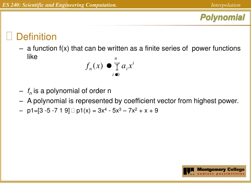
Polynomial. Definition a function f(x) that can be written as a finite series of power functions like f n is a polynomial of order n A polynomial is represented by coefficient vector from highest power. p1=[3 -5 -7 1 9] p1(x) = 3x 4 - 5x 3 – 7x 2 + x + 9. Polynomial Operations.

E N D
Polynomial • Definition • a function f(x) that can be written as a finite series of power functions like • fnis a polynomial of order n • A polynomial is represented by coefficient vector from highest power. • p1=[3 -5 -7 1 9] p1(x) = 3x4 - 5x3 – 7x2 + x + 9
Polynomial Operations • poly(r) • convert roots to a polynomial • r=[ 1 2 3 ]; poly(r) • roots(p) • find roots of a polynomial • p=[ 2 3 4 ] • roots(p) • Y = polyval(p, x) • returns the value of a polynomial, p(x). • P is a vector of length N+1 whose elements are the coefficients of the polynomial in descending powers. • p=[3 -5 -7 1 9] p(x) = 3x4 - 5x3 – 7x2 + x + 9
Polynomial Operations • P = polyfit(x, y, n) • Returns the least squares fit coefficients of a polynomial p(x) of degree n • P is of length N+1. • conv(p1,p2) • multiply two polynomials p1 and p2 • conv(p1,p2) • [q r]=deconv(p1,p2) • polynomials p1 divide by p2, where q is quotient and r is remainder • [q r]=deconv(p1,p2)
Polynomial Operations • polyint(p,c) • integrate of polynomial p with integration constant c (default 0) • polyint(p) • polyint(p,1) • polyder(p) • differentiate polynomial p respective to x • >> polyder(p)
Curve Fitting • Applications • Estimating the value of points between discrete values • Simplifying complicated functions • Methods • Interpolation • Data are very precise • curve passes through all points • curve fitting • Data are just approximations • curve represent a general trend of the data
Curve Fitting and Interpolation Curve Fitting (linear or non-linear) Linear Interpolation (most popular interpolation) Other Interpolation (higher order polynomial, spline, nearest,…)
Linear Interpolation • The linear interpolation is achieved by fitting a line between two known data points • The resulting formula based on known points x1 and x2 and the values of the dependent function at those points is:
Quadratic (Polynomial) Interpolation • One problem that can occur with solving for the coefficients of a polynomial is that the system to be inverted is in the form: • Matrices such as that on the left are known as Vandermonde matrices, and they are very ill-conditioned - meaning their solutions are very sensitive to round-off errors. • The issue can be minimized by scaling and shifting the data.
Newton Interpolating Polynomials • Another way to express a polynomial interpolation is to use Newton’s interpolating polynomial. • This is a achieved by an extension to linear interpolation
Newton Interpolating Polynomials (cont) • The second-order Newton interpolating polynomial introduces some curvature to the line connecting the points, but still goes through the first two points. • The resulting formula based on known points x1, x2, and x3 and the values of the dependent function at those points is:
Generalization • An (n-1)th Newton interpolating polynomial has all the terms of the (n-2)th polynomial plus one extra. • The general formula is:where and the f[…] represent divided differences.
Divided Differences • Divided difference are calculated as follows: • Divided differences are calculated using divided difference of a smaller number of terms:
Example 15.1 Do by hand Use the newtint function
Lagrange Interpolating Polynomials • Weighted average of the two values being connected • The differences between a simple polynomial and Lagrange interpolating polynomials for first and second order polynomials is: • where the Li are weighting coefficients that are functions of x.
Lagrange Interpolating Polynomials (cont) • The first-order Lagrange interpolating polynomial may be obtained from a weighted combination of two linear interpolations, as shown. • The resulting formula based on known points x1 and x2 and the values of the dependent function at those points is:
Lagrange Interpolating Polynomials (cont) • In general, the Lagrange polynomial interpolation for n points is: • where Li is given by:
Example 15.1 Solve by hand Use the lagrange function
Extrapolation • Extrapolation is the process of estimating a value of f(x) that lies outside the range of the known base points x1, x2, …, xn. • Extrapolation represents a step into the unknown, and extreme care should be exercised when extrapolating!
Extrapolation Hazards • World population using a 7th order polynomial extrapolation.
Oscillations • Higher-order polynomials can not only lead to round-off errors due to ill-conditioning, but can also introduce oscillations to an interpolation or fit where they should not be. • In the figures below, the dashed line represents a function, the circles represent samples of the function, and the solid line represents the results of a polynomial interpolation:
Introduction to Splines • An alternative approach to using a single (n-1)th order polynomial to interpolate between n points is to apply lower-order polynomials in a piecewise fashion to subsets of data points. • These connecting polynomials are called spline functions. • Splines minimize oscillations and reduce round-off error due to their lower-order nature.
Higher Order vs. Splines • Splines eliminate oscillations by using small subsets of points for each interval rather than every point. This is especially useful when there are jumps in the data: • 3rd order polynomial • 5th order polynomial • 7th order polynomial • Linear spline • seven 1st order polynomials generated by using pairs of points at a time
Spline Development • First-order splines find straight-line equations between each pair of points that • Go through the points • Second-order splines find quadratic equations between each pair of points that • Go through the points • Match first derivatives at the interior points • Third-order splines find cubic equations between each pair of points that • Go through the points • Match first and second derivatives at the interior pointsNote that the results of cubic spline interpolation are different from the results of an interpolating cubic.
Spline Development • Spline function (si(x))coefficients are calculated for each interval of a data set. • The number of data points (fi) used for each spline function depends on the order of the spline function.
Cubic Splines • While data of a particular size presents many options for the order of spline functions, cubic splines are preferred because they provide the simplest representation that exhibits the desired appearance of smoothness. • In general, the ith spline function for a cubic spline can be written as: • For n data points, there are n-1 intervals and thus 4(n-1) unknowns to evaluate to solve all the spline function coefficients. • There is no ‘one equation’ that can represent the whole spline function on the domain
Piecewise Interpolation in MATLAB • MATLAB has several built-in functions to implement piecewise interpolation. The first is spline:yy=spline(x, y, xx) • This performs cubic spline interpolation
Example • Generate data:x = linspace(-1, 1, 9);y = 1./(1+25*x.^2); • Calculate 100 model points anddetermine not-a-knot interpolationxx = linspace(-1, 1);yy = spline(x, y, xx); • Calculate actual function values at model points and data points, the 9-point (solid), and the actual function (dashed), yr = 1./(1+25*xx.^2)plot(x, y, ‘o’, xx, yy, ‘-’, xx, yr, ‘--’)
MATLAB’s interp1 Function • While spline can only perform cubic splines, MATLAB’s interp1 function can perform several different kinds of interpolation:yi = interp1(x, y, xi, ‘method’) • x & y contain the original data • xi contains the points at which to interpolate • ‘method’ is a string containing the desired method: • ‘nearest’ - nearest neighbor interpolation • ‘linear’ - connects the points with straight lines • ‘spline’ - not-a-knot cubic spline interpolation • ‘pchip’ or ‘cubic’ - piecewise cubic Hermite interpolation
Lab • 15.9