Download
1 / 72
771 likes | 986 Views
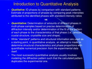
Introduction to Quantitative Skills/Graphing. August 19, 2014. Objectives. Students need to be able to determine what type of graph (e.g., histogram, line graph) most appropriately reflects their collected data and then

E N D
Introduction to Quantitative Skills/Graphing August 19, 2014
Objectives Students need to be able to determine what type of graph (e.g., histogram, line graph) most appropriately reflects their collected data and then create the graph and use it to draw conclusions, make predictions, and pose questions for further investigation. • Mean, median, mode, range • The nature of science • Observations vs. Inferences • Populations vs. Samples • Null vs. Alternative Hypotheses • Designing an Experiment • Graphing • Basic Statistics
Review • Mean: average of a set of numbers • Median: middle number if you add them up smallest to largest • Mode: most frequent number • Range: largest number minus smallest number
Mean, Median, Mode, Range Example 13, 18, 13, 14, 13, 16, 14, 21, 13
Nature of Science • Science is about finding answers to problems through investigations • Science is about questioning everything (skepticism). Don’t tell me something is true, prove it to me! • Science is about only accepting something as the “right answer” if enough evidence has been built to support it and it can be replicated by others • There is no emotions in science….but… • Creativity is a vital, yet personal, ingredient in the production of scientific knowledge.
The Science Community • The science community questions findings, replicates hypotheses, and peer reviews publications • By it’s very nature, the science community is a scientists biggest critic • Real debates should be between two parties who both hold massive amounts of evidence
Science is Dynamic Scientific knowledge is simultaneously reliable and tentative. Having confidence in scientific knowledge is reasonable while realizing that such knowledge may be abandoned or modified in light of new evidence or reconceptualization of prior evidence and knowledge
Examples of Science Gone Wrong • Is the earth the center of the universe? Is the earth flat? • Newton’s three laws of motion – considered fact until we got into Einstein's Theory of Relativity • Even NASA was wrong!
The Nature of Science • It’s also just as bad to ignore mounting evidence against virtually undisputed scientific theories • Evolution • Global Warming • The nature of science is to QUESTION, CHALLENGE, BE OBJECTIVE, and THINK CRITICALLY • It’s OK to change your mind!
Basis of the Scientific Method • It’s okay if your hypothesis is wrong!!!! • Your experimental design is critical! • ALL scientists must be FLUENT in statistics • If your data supports your hypothesis, does that mean your conclusion is fact? Hmmm • There are NO facts in science. Whhhaaa?
Observation vs. Inference • Observation: using your five senses to observe descriptive things • Qualitative • Quantitative • Inference: taking all of the observations you have made and trying to explain them • You do this every day, whether you are meaning to or not
Observations lead to questions • We make observations everyday with our senses • Qualitative: descriptive (The cat is grey) • Quantitative: numerical (The cat weighs 22 lbs) • A gathering of sample observations help us make inferences about populations with our reasoning skills • We can never know anything for sure about the true population – it is often too large and ever changing
Evidence • Scientists must generate data as evidence • Data can be: • Quantitative: numbers, data measured, uses instruments • Qualitative: descriptive, data observed, uses senses
Quantitative Data • Can be either: Continuous of Discrete
Quantitative data you collect will fall into 1 of 3 categories • Parametric data • Normal curve = bell curve = parametric data • Describes most populations • usually decimals included (continuous) • The less bias your sample is, the closer to the true mean it will be • Nonparametric data • not normally distributed (bell-shaped) • includes outliers • Qualitative (small, medium, large) • Frequency/count data • Ex. How many flies with certain type of wing • This is a way to make qualitative data quantitative data
Non-Parametric Data • Generally, the parameters calculated for nonparametric statistics include medians, modes, and quartiles, and the graphs are often box-and-whisker plots • Why would we use medians instead of means for non-parametric data?
Formulating Hypotheses • Null hypothesis (Ho): No observed effect; the opposite of what you’re testing • Alternative hypothesis (HA) or (H1): An effect was observed; the claim your testing • We either fail to reject the null () or reject the null () • To begin with we always assume the null is true (like innocent until proven guilty) • As a scientist, the alternative hypothesis is our friend and being able to reject the null is very exciting because if a significant effect was observed then we get to publish our results!
Examplein #’s • (Ho): μ< 2.7 • (HA): μ > 2.7 • (Ho): • (HA): Examplein words
Designing an Experiment • Variables • Independent: what we control/change • Dependent: what changes in response to independent • Constant Variable – variables that remain unchanged so we can accurately test out dependent variable • Control Group • Sample of our population (N) must be LARGE & RANDOM • Repeated Measures “___(blank)___ depends on ___(blank)___”
Identify the experimental parameters • Independent Variable: • Dependent Variable: • Control Variable: • Control Group:
Tables and Graphs • A graph is a visual representation of a data set • On your AP test you will be given a data table and must decide which type of graph will be used • What’s the difference between a bar graph and a histogram? Histogram
Bar Graphs • Use two compare two samples of categorical or count data. You will need to compare the calculated means with error bars. Example: qualitative: eye color. Always use Sample Standard error bar. (Sample error of the mean) (SEM)
Scatterplots • Used to explore associations between two variables visually. One variable is measured against another. It is looking for trends or associations. Plotting of individual data points on an x-y plot.
Scatterplots • Sine wave-like Bell-curved
Box-and-whisker plot • Allows comparison of two samples of nonparametric data (data that does not fit a normal distribution) • Medians and quartiles
Histogram - nonparametric • For frequency data • Can turn numbers into categories!
Cheat sheet of what type of graph to use when • Pie charts are you to represent percentages of categorical data mostly, but they have a major downfall: they cannot present the error • Only if you are graphing rate (something changing over time), than you will do a line graph • Rate equals “rise over run” or the slope of the graph • If you have frequencies of a number range histogram • Use bar graph when one variable is categorical, and one is numerical • Use scatterplot when both variables are numerical and you want to see a trend (best fit line)
Don’t lose points! • Be neat! • Don’t forget a TITLE: usually same as the table title it is representing • LABEL AXES: dependent variable goes on y-axis; independent goes on the x-axis • Numbers should ascend from bottom to top or from left to right • Numbers of axes must be EVENLY spaced • Don’t necessary have to start data at origin…explanation?
Interpreting General Curves of Graphs • Bell-shaped curve: associated with random samples and normal distributions. • Concave upward curve: associated with exponentially increasing functions (for example, in the early stages of bacterial growth) and then plateauing upon saturation/carrying-capacity • A sine wave–like curve: is associated with a biological rhythm
The Importance of Standard Error • Ho: There is no difference between McDonalds & Wendy’s • HA: There is a difference between McDonalds & Wendy’s
Statistics is the Basis of Science! • Statistics is the MOST important math in Ms. Grapes’ opinion • If you are going into a science-based career, take it! • Even if you are not, knowing statistics will help you think quantitatively, AKA make better life decisions and think for yourself.
Determining Significance • How can we tell if we accept or reject Ho? AKA How do we know when the differences we see in data are significant? • In simple statistics we need two things • The average • The standard deviation (σ or s) • You can be accurate without being precise
Empirical Rule • The Empirical Rule/67-95-99.7 Rule/three sigma rule describes the bell curve • 95% confidence interval: a measure of the reliability of an estimate
Standard Error vs. Standard Deviation • Standard error allows for inference of how sample mean matches up to the true population mean. • A distribution of the sample means helps define boundaries of confidence in our sample. 1 SE describes 67% confidence range. 2 SE defines 95% certainty Confidence limits contains the true population mean. 95% confident: larger range to contain the population mean(95% of the data found here) 67% confident: narrower range to contain the population mean. SE – inference in which to draw conclusions SD – just looking at data 95% is trade off for never being 100% sure.
From AP A sample mean of ±1 SE describes the range of values about which an investigator can have approximately 67% confidence that the range includes the true population mean. Even better, a sample with a ±2 SE defines a range of values with approximately a 95% certainty. In other words, if the sampling were repeated 20 times with the same sample size each time, the confidence limits, defined by ±2 SE, would include the true population mean approximately 19 times on average. This is the inference; it is a statistic that allows investigators to gauge just how good their estimate of the true population mean actually is.
Best-fit line, linear regression, and r • A best fit line indicates the general trend • A regression line is a best fit line that summarizes all the points into a single linear equation…for scatterplot • Positive correlation/direct relationship: both variables go up together • Negative correlation/Indirect relationship: as one variable goes up, the other gown down. • r-value (from -1 to 1) • provides an estimate of the degree of correlation. • 0 equals no correlation • 1 is a perfect positive correlation and -1 is visa versa
Standard Deviation (σ) • The average value away from the average • The smaller σ, the better • If your results were ‘precise’ you will have a small std. dev. • The standard deviation is the square root of the variance http://www.mathsisfun.com/data/standard-deviation.html