Download
1 / 34
400 likes | 548 Views
Brownian Motion. Einstein’s “Miracle Year”: 1905 (Berne, Switzerland). March 1. “On a Heuristic Point of View Concerning the Production and Transformation of Light” April 2. “A New Determination of Molecular Dimensions” May 3. “On the Movement of Small Particles Suspended

E N D
Einstein’s “Miracle Year”: 1905 (Berne, Switzerland) March 1. “On a Heuristic Point of View Concerning the Production and Transformation of Light” April 2. “A New Determination of Molecular Dimensions” May 3. “On the Movement of Small Particles Suspended in a Liquid Demanded by the Molecular Kinetic Theory of Heat”
Einstein’s “Miracle Year”: 1905 (Berne, Switzerland) June 4. “On the Electrodynamics of Moving Bodies” September 5. “Does the Inertia of a Body Depend on Its Energy Content? December 6. “On the Theory of Brownian Movement”
The contradiction Einstein pointed out • For liquid solutions, osmosis is well-understood: the • semipermeable membrane is pushed by random • motion of solute molecules, to the right • No such effect expected for piles of rocks and sand!!
How Einstein thought it out • p(x) = pressure at a point and c(x) = molar concentration • of the dissolved solute at a point x in 1d [c = number of • moles/volume = n/V] • IF the SOLUTE IS DILUTE IT ACTS LIKE AN IDEAL • GAS, SO pV = nRT becomes p = RTc • This quantity varies from point to point nothing more or • less than the osmoticpressure
The force per unit volume is minus the pressure gradient at a point • dp = p(x + dx) - p(x) = (tiny) difference in pressure between x + dx and x • force = pressure x area, so F(x) = p(x) A • (tiny) volume dV = A dx of solution (solute molecules) in the slice • dx feels a net osmotic force dF= - A dp • the force per unit volume f = dF/dV = - dp/dx • f = minus spatial derivative of the pressure: gradient!!
Now to let this force push a molecule • Recall that p = RTc so • What is the volume w of one solute molecule? • since c = number of moles/volume . . . • 1/c = volume per mole = NAw w = 1/ NAc • so: the osmotic force on a molecule fo is osmotic force per unit • volume times the volume w: • Osmosis pushes molecules from high to low concentration
Include viscous drag force too • Assume molecule is a sphere of radius r • viscous drag force fd on the solute molecule proportional to its • speed v and to solvent viscosity h • specifically, according to Stokes’s law: fd = - 6phrv • in equilibrium, these two forces are balanced: • this is version 1 of D: in terms of simple system #s • units of vc: (m/s)(moles/m3)=moles/area•time • The left side is therefore is a “mole flux rate”
Diffusion as mole flux rate • Consider the time t, in which molecules • move “typical” distance D to R or L • t is LARGE compared to intercollision time, • but SMALL compared to system • equilibration time • The number of moles that pass the central slice to R • in time t is (half move L and half move R) • The number of moles that pass the central slice to • L in time t is
Diffusion Confusion continued • the net number moving to R is the difference: • But • the net number moving to R becomes • So, dividing by the area A and the time t gives the mole flux rate again, as • Einstein thus derives version 2: D = D2/2 t • Notice that he’s managed to avoid use of v !!
Diffusion Conclusion • Equate these two versions of D • This is part of the remarkable conclusion: the typical distance D traveled in time t is not LINEAR in t but varies like (slower-growing) t1/2 • If the solute is tiny, then so is r, and things zip around too fast to observe • But if the “solute” is huge, like a pollen grain, then the distance traveled is smallish and you might “see” it move, in the sense of “where it is” as time goes by without needing “how fast it moves”
Diffusion or Heat Equation aside • The classical diffusion equation governs how concentrations of stuff diffuse away in x and t • The solution is a Gaussian function in space that slowly flattens out as time goes by • The conventional versions are these: • Well-understood by the 19th century crowd • Einstein derives this in his paper • He “points out” that observations of pollen grains can lead to a way to measure NA!!!
Features of the Gaussian • area under curve is proportional at any t to the amount of “stuff” • <x> = 0 = mean value • D = <x2>= 2Dt = peak’s “width” = standard deviation • describes concentration decay of an initial infinitely spiked distribution of stuff at t = 0 • describes all kinds of other phenomena too: if you know the mean and the standard deviation you know everything you need to know
The Gaussian Probability Distribution Red: t =50 Blue: t = 500 Green: t =5000
The Random Walk in one dimension (A drunken mole leaves its hole . . .) • Assume a step size 1, with equal probability to L or R • After total of N steps, mole is at position m • m may be + or - ; clearly, |m|scales with N • One might guess that m ~ N but that is wrong! • Let Np = number of steps to R, Nn = number to L, so clearly N = Np + Nn and m = Np - Nn • These two equations can be easily solved, to obtain
Combinatorics: let me count the ways • We are interested in P(m,N): the probability that after N steps, the mole is at position m • Elementary combinatorics tells us that the number of distinct ways of pulling (say) b different balls from a total of B different balls is given by (! = the factorial operation) Example: given 5 balls (A, B, C, D, E), how many distinct ways can we pull three balls? ABC ABD ABE ACD ACE ADE BCD BCE BDE CDE And 5!/(3!)(2!) = 120/(6)(2) = 120/12 = 10
Probability P(m,N) • P(m,N) is equal to the number of ways of getting to position mtimes the probability of that way • a “way”is a specific unique sequence of N steps that takes the mole to m (like LLRLRRLRRLLLRLRR …)
Stirling’s Method • N is a gigantic number in life (the step size is tiny) and, even worse, N ! is beyond comprehension • logarithms are a way to tame huge numbers • Stirling’s approximation for the factorial: if N is large • N = 20: 20 ! = 2.433 x 10¹⁸ ln (20 !) = 42.336… • 42.336 = (20.5)ln 20 - 20 + .919 • 42.336 = 61.413 - 20 + .919 = 41.413 + .919 = 42.332
The Gaussian Probability Distribution • After a lot of algebra, many things simplify • We assume that m << N too, which is bold but true! • Now we can “exponentiate” both sides • This result is the same as the diffusion equation solution!! Recall . . .
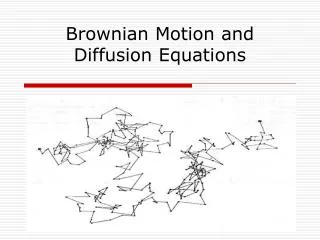
The connection to diffusion • so x is just m: distance from home • and 2Dt is just N which is D2 (width2) (Einstein result) • After N steps, the mole has reached a “typical distance” D of perhaps D = N from home • It’s unlikely to be more than 2D or 3D from home • As is characteristic of all random walks, this “typical” distance ~ N [SAME BIG SURPRISE!] • Things are much the same in 2d and 3d • Brownian motion is just a “random walk” in 3d
Other approaches to stochastic problems Fokker-Planck Equations: Norbert Wiener’s theory of stochastic processes Image of Langevin: Wolfram Research Image of Fokker: Huygens-Fokker Foundation Others: American Institute of Physics
Chandrasekhar’s contributions • Derived W from its limiting forms: must be a delta function as t 0, and a Maxwellian as t • from r – ro = v(t) dt, for t . . .
Applications by Chandra and others • Treated various forms of external force • Analyzed the “short-time” behavior • Average time of recurrence of a fluctuation • Colloid statistics • Sedimentation in gravity • Star dynamics (random gravity) • Radiation diffuses: led to famed 1.4 M☼ cutoff for supernova . . • Predictability of the stock market • Predictability of Earth’s climate • Theory of noisy information
The self-avoiding random walk • 1d: trivial • 2d: solvable • 3d: not yet solved: application to polymers and protein folding problem
Uncorrelated vs. sort of correlated Pure Brownian motion: next step is uncorrelated with previous step Persistent Fractional Brownian motion: each step is positively correlated with previous step Anti-Persistent Fractional Brownian motion: each step is negatively correlated with previous step
Pretty pictures of things that don’t exist Alexis Brandecker Berndt M. Gammel Make it move http://www.astro.su.se/~alexis/fractals/Cloud3D.gif
Some history behind Brownian motion • The discovery of ‘Brownian motion’ is attributed to the botanist Robert Brown. In • 1827, Brown noticed the irregular motion of pollen particles suspended in water, and • was able to rule out the motion being due to the pollen being ‘alive’ by repeating the • experiment using suspensions of dust in water. However, at the time, the origin of this • Brownian motion could not be explained. • The first explanation of the mathematics behind Brownian motion was made by • Thorvald Thiele in 1880 (the mathematics of Brownian motion is important in fields • ranging from fractals to economics).
Some history behind Brownian motion • However, it was Albert Einstein who is widely acknowledged for putting together the • first physical understanding of Brownian motion in 1905. At the time, the atomic • nature of matter was still controversial, so understanding that Brownian motion was • due to the kinetic motion of particles was an important result. In fact, it was one of • two results that earned Einstein the Nobel Prize in 1921, and one of Einstein’s three • great discoveries in 1905. • Finally, Jean Perrin carried out the first experiments to test the new mathematical and • theoretical models for Brownian motion, as we’ll see later. The results of this ended a • 2000-year-old dispute (beginning with Democritus and Anaxagoras in ~500 B.C.) • about the reality of atoms and molecules.
Some history behind Brownian motion • Brownian motion is also very important • in biology, where you have a lot of small • molecules and structures immersed in • water at ~300K, and is even used by • biological entities to move things • around. If you’re interested, see this • week’s reading “Making molecules into • motors” by R. Dean Astumian from • Scientific American.
Some history behind Brownian motion • Brownian motion is also very important • in biology, where you have a lot of small • molecules and structures immersed in • water at ~300K, and is even used by • biological entities to move things • around. If you’re interested, see this • week’s reading “Making molecules into • motors” by R. Dean Astumian from • Scientific American. • The Concept • Imagine you are at the cricket. The crowd gets a bit bored so they pull out a large • beach ball and start bouncing it around. As you know, assuming someone isn’t • deliberately aiming it in some direction (like away from security), it will take a random • path through the crowd. • • If the ball is a few seat-areas away, it may seem that • the ball never seems to make it over to you. Instead, it • just wanders ‘around in circles’ near where it started, • travelling a long path but not travelling very far from • its origin. • • This is very similar to Brownian motion, but here the • ball only takes one hit at a time with some long • interval in between. In Brownian motion, the hits are • more frequent, so let’s extend our analogy a little • further.
Some history behind Brownian motion • • Imagine that the beach-ball is actually really big, say 20 m in diameter (not 1 m in • diameter like the one in the picture last slide). This ball will be so big that many • people in the crowd can hit it all at once. • • If we now consider the force on it, 20 people might be pushing it to the left and 21 • people might be pushing it to the right, so the forces to the left and right are • almost balanced and there is a small net force to the right, and the ball will take a • small step right. Next time, it might go another direction. • • The motion will be even more random now, one person might want to send it some • direction, but on average that will be cancelled out by all the other directions that • people are pushing it in, and so at each point the net force on the ball will be • random, and the strength and direction of the net force will depend entirely on the • balance of all the little pushes that it receives
Brown’s experiment – Pollen in water • • Returning to Robert Brown’s experiment in 1827 – the motion of pollen in water – the • physics is pretty much the same. • • A liquid is just a gas where the potential energy between the particles is comparable • to the kinetic energy of those particles (in contrast a gas has negligible potential • energy compared to the kinetic energy and the particles travel around freely between • collisions). • • So the particles of the liquid are all bouncing around (just very close to each other • and making lots of collisions with one another) and if we stick a piece of pollen in, we • get something very close to our beach ball analogy – a lot of water particles smacking • against the pollen particle and randomly pushing it around. • • The water particles are ~1 nm in size, and our pollen particle is ~ 1μm, about 1000 • times bigger (given a fist is about 10 cm in diameter, this would mean a beach-ball • around 100 m in diameter!). So the pollen particle would receive a massive quantity of • little pushes (about 1014 per s) from all the water molecules bouncing against it, and at • any time the net force would be the balance of all these little pushes.
Brown’s experiment – Pollen in water • • Returning to Robert Brown’s experiment in • • The experiments can be tricky (watching tiny particles for long periods under a • microscope) but we can quite easily see the behaviour of a particle undergoing • Brownian motion using simulations: • http://www.chm.davidson.edu/ChemistryApplets/KineticMolecularTheory/Diffusion.html • and • http://mutuslab.cs.uwindsor.ca/schurko/animations/brownian/gas2d.htm • • In the simulations, the pollen particle wanders about randomly, and each time, the • path is completely random and different. The one consistent thing is that as the • particle wanders around, the ‘spread’ of its path away from the starting point slowly • increases with time. • • It’s also clear that the particle travels a much smaller distance than we’d expect if it • was just travelling along at its velocity. • • So a very useful question to ask at this point is: After a given length of time, how far • away from its starting point is the particle likely to be? This is exactly the question • that Einstein and Smoluchowski asked in 1905