Download
1 / 59
590 likes | 911 Views
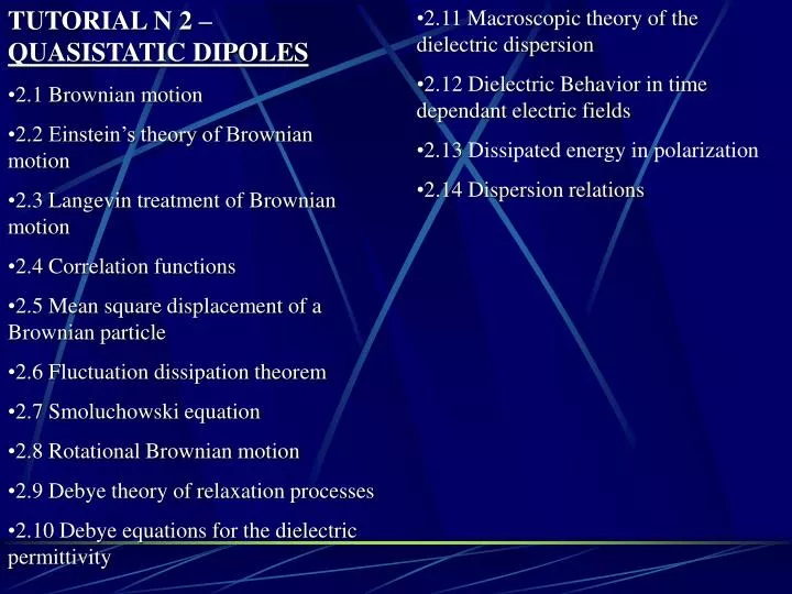
TUTORIAL N 2 – QUASISTATIC DIPOLES 2.1 Brownian motion 2.2 Einstein’s theory of Brownian motion 2.3 Langevin treatment of Brownian motion 2.4 Correlation functions 2.5 Mean square displacement of a Brownian particle 2.6 Fluctuation dissipation theorem 2.7 Smoluchowski equation

E N D
TUTORIAL N 2 – QUASISTATIC DIPOLES • 2.1 Brownian motion • 2.2 Einstein’s theory of Brownian motion • 2.3 Langevin treatment of Brownian motion • 2.4 Correlation functions • 2.5 Mean square displacement of a Brownian particle • 2.6 Fluctuation dissipation theorem • 2.7 Smoluchowski equation • 2.8 Rotational Brownian motion • 2.9 Debye theory of relaxation processes • 2.10 Debye equations for the dielectric permittivity • 2.11 Macroscopic theory of the dielectric dispersion • 2.12 Dielectric Behavior in time dependant electric fields • 2.13 Dissipated energy in polarization • 2.14 Dispersion relations
d - - - - E - - + + + + + + Lorentz local field
Claussius – Mossotti equation valid for nonpolar gases at low pressure. This expression is also valid for high frequency limit. The remaining problem to be solved is the calculation of the dipolar contribution to the polarizability.
By substituting Eq (1.9.3) into Eq (1.9.12) and taking into account Eq(1.9.2), one obtain Debye equation for the static permittivity
According to Onsager, the internal field in the cavity has two components: • 1 – The cavity field, G, (the field produced in the empty cavity by the external field.) • 2 - The reaction field, R (the field produced in the cavity by the polarization induced by the surrounding dipoles).
Onsager treatment of the cavity differs from Lorentz’s because the cavity is assumed to be filled with a dielectric material having a macroscopic dielectric permittivity. • Also Onsager studies the dipolar reorientation polarizability on statistical grounds as Debye does. • However, the use of macroscopic argument to analyze the dielectric problem in the cavity prevents the consideration of local effects which are important in condensed matter. • This situation led Kirkwood first, and Fröhlich later on the develop a fully statistical argument to determine the short – range dipole – dipole interaction.
Claussius – Mossotti: Only valid for non polar gases, at low pressure • Debye: Include the distortional polarization. • Onsager: Include the orientational polarization, but neglected the interaction between dipoles. describe the dielectric behavior on non-interacting dipolar fluids • Kirkwood: include correlation factor (interaction dipole-dipole) • Fröhlich – Kirkwood – Onsager
2.1. Brownian Motion • Many processes in the nature are stochastic. • A stochastic process is a set of random time-dependent variables. • The physical description of a stochastic problem requires the formalization of the concept of „probability”, and „average” • A Markov process is a stochastic process whose future behavior is only determined by the present state, not the earlier states. Brownian motion is the best-know example of Markov process.
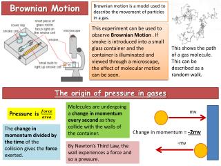
Robert Brown • British Botanist (1773 – 1858). • In 1827, while examining pollen grains and the spores suspended in water under a microscope, observed minute particles within vacuoles in the pollen grains executing a continuous jittery motion. • He then observed the same motion in particles of dust, enabling him to rule out the hypothesis that the motion was due to pollen being alive. • Although he himself did not provide a theory to explain the motion, the phenomenon is now known as Brownian motion in his honor.
Brownian motion refers to the trajectory of a heavy particle immersed in a fluid of light molecules that collide randomly with it. • The velocity of the particle varies by a number of uncorrelated jumps. • After a number of collisions, the velocity of the particle has a certain value v, The probability of a certain change v in the velocity depends on the present value of v, but not on the preceding values. An ensamble of dipoles can be considered a Brownian system. • Einstein made conclusive mathematical perdictions of the diffusive effect arising from the random motion of Brownian particles bombarded by other particles of the surrounding medium. • Eintein’s idea was to combine the Maxwell-Boltzmann distribution of velocities with the elementary Markov process known as random walk.
The random walk model is used in many branches of physics. Particularly can be used to describe the molecular chains of amorphus polymers. The probability distribution function for end-to-end distance R of freely jointed chains can be obtained by solving: (Simplest case of probability density diffusion equation Focker – Plank Equation) Parabolic differential equation is the same for other random walk phenomena as heat conduction or diffusion where P is the probability distribution, b is the length of each segment, and n is the number of bonds. It is also assumed that n>>1, and R>>b. The solution under the condition that R is at the origing when n=0,
2.2 EINTEIN’S THEORY OF BROWNIAN MOTION • If a particle in a fluid without friction collides with a molecule of the fluid, its velocity changes. • However, if the fluid is very viscous, the change in the velocity is quickly dissipated and the net result of the impact is a change in the position of the particle. • Thus what is generally observed at intervals of time in Brownian motion is the displacement of the particle after many variation in the velocity. • As a result, random jumps in the position of the particle are observed. • This is a consequence of the fact that the time interval between the observation is larger than the time between collisions. • Accordingly, the kinetic energy of translation of a Brownian particle behaves as a non-interactive molecule of gas, as required in the kinetic elementary theory of gases.
Assuming very small jumps, Einstein obtained the probability of distribution of the displacement of particles the following partial differential equation: • D: Diffusion coefficient, <x2> mean-square displacement, time interval such that the motion of the particle at time t is independent of its motion at time t+ • Using the Maxwell distribution of velocities, the diffusion coefficient is obtained as: • Where, T is the temperature, k, the Boltzmann constant and the friction coefficient
2.3 LANGEVIN TREATMENT OF THE BROWNIAN MOTION • Langevin introduce the concept of equation of motion of a random variable and initiated the new dynamic theory of Brownian motion in the context of stochastic differential equations. Langevin’s approach is very useful in finding the effect of fluctuations in macroscopic systems. • Langevin equation of motion of a Brownian particle start from the Newton’s second law and two assumptions: • (1) the Brownian particle experiences a viscous force that represent a dynamic friction given by • (2) a fluctuating force F(t), due to the impacts of the molecules of the surrounding fluid on the particle in question appears. The force fluctuates rapidly and is called white noise
The friccion force is governed by Stokes’ law. The expresion for the friccion coefficient of a spherical particle of radius a and mass m, moving in a medium of viscocity is The force F(t) is unpredictalbe, but it is clear that the F(t) may be treated as a stochastic variable (its mean value vanishes).
2.4 CORRELATION FUNCTIONS • A correlation is an interdependence between measurable random variables. We consider processes in which the variables evaluated at different time are such that their stochastic properties do not change with time. This processes are said to be stationary and the correlation function between two variables in these processes is expressed by • An autocorrelation function is a correlation function of the same variable at different times, that is
The normalized autocorrelation function is expressed as • Due to the fact that the random force F(t), is caused by the collisions of the molecules of the sourrounding fluid on the Brownian particle, we can write • Where is a contant and (t) the Dirac delta function. Eq. 2.4.4, express the idea that the collisions are practically instantaneous and uncorrelated. It also indicates that F(t) is a white spectrum. Eq. 2.4.4 can be written as
2.5 MEAN-SQUARE DISPLACEMENT OF A BROWNIAN PARTICLE • By multiplying both sides of Eq. 2.3.1 by x(t), and taking into account that • Averaging over all the particles, and assuming that the Maxwell distribution of velocities holds, that is
Note that <Fx>=0 since the random force in uncorrelated with the displacement. • Substituing the expression 2.5.5 in Eq 2.5.4 • Whose solution is • And K is an integration constant. For long times, or friction constants larger than the mass, the exponential term has no influence on the motion of the particle after some time interval. This is equivalent to excluding inertial effects, in these conditions, we have
Integrating the Eq. 2.5.8, from t=0 to t=, and assuming that x=0 for t=0, we obtain • This is the same result obtained by Einstain.
2.6 FLUCTUATION-DISSIPATION THEOREM • The Langevin equation can also be solved for the velocity, taking into account that x’=v. • Where v(0)=vo. By averaging this equation for an ensemble of particles, all having the same initial velocity vo, and noting that the noise term F(t’) is null in average and uncorrelated with velocity, we obtain
Squaring the expr 2.6.1, and further integration on the resulting expression leads to • is given by the expression 2.4.4 and it was taken into account that <F(t).F(t’)>=(t-t’). • In order to identify , we note that for t →∞, eq 2.6.3 becames • The Eq. (2.6.4) relates the size of the flucuacting term , to the damping constant . In other words, fluctuactions induce damping. This is the first version of the fluctuation – dissipation theorem, whose main relevant aspect is that it relate the microscopic noise to the macroscopic friction. • According to van Kampen: „The physical picture is that the random kiks tend to spread out v, while the damping term tries to bring v back to zero. The balance between these two opposite tendencies is the equilibrium distribution”
2.7 SMOLUCHOWSKI EQUATION • A further step in the approach to Brownian motion is to formulate a general master equation that model more accurately the properties of the particles in question. Eq 2.2.1 can be written as a continuity equation for the probability density Where j is the flux of Brownian grain or, in general, the flux of events suffered by the random variable whose probability density has been designed as f. Part of this flux is diffusive in origin and, according to a first constitutive assumption, can be written as
D is the diffusion coefficient given by kT/. • Now we introduce a second constitutive assumption. Let us to suppose that the particles are subject to an external force that derive of a potential function, so that • Then, the current density of the particles that is due to this external force can be expressed as • If the external foce is related to the velocity through the equation the drift current due to this effect will be
The sum of two current fluxes (j=jdiff+jd) and the substitution into Eq. (2.7.1) yields Smoluchowski Eq. diffusiveconective (transport or drift term)
2.8 ROTATIONAL BROWNIAN MOTION • The arguments used to establish the Smoluchowski equation can be applied to the rotational motion of a dipole in a suspension. • In this case the fluctuating quantity is the angle or angles of rotation. • The Debye theory of dielectric relaxation has as its starting point a Smoluchowski equation for the rotational Brownian motion of a collection of homogeneous sphere each containing a rigid electric dipole , where the inertia of the spheres is neglected. • The motion is due entirely to random couples with no preferential direction. • We take at the center of the sphere a unit vector u(t) in the direction of . • The orientation of this unitary vector is described only in terms of the polar and azimuthal angles and . Having the system spherical symmetry, we must to take the divergence of Eq. (2.7.1) in spherical coordinates, that is
The current density contains two terms, a diffusion term defined in Eq. (2.7.2) given in spherical coordinates by Where e and e, are unit vector corresponding to the and coordinates, and the term f(,,t) represent the density of dipole moment orientation on a sphere of unit radius. On the other hand, the convective contribution to the current is due to the electric force field acting upon the dipole. The corresponding equation for such current is similar to Eq. (2.7.6) but now U is the potential for the force produced by the electric field. This force can be calculated by combining the kinematic equation for the rate of change in the unity vector u, given by With the noninertial Langevin equation for the rotating dipole, that is
where Fis the white noise driving torque and μ x E is the torque due to an external field. For this reason, between two impacts, Eq (2.8.4) can be written as • This is, the angular velocity of the dipoles under the effect of the applied field Eq. (2.8.4)is the differential equation for the rotational Brownian motion of a molecular sphere enclosing the dipole μ. Introduction of Eq (2.8.4)into Eq (2.8.3)yields • Equation (2.8.6)is the Langevin equation for the dipole in the noninertial limit. The applied electric field is the negative gradient of a scalar potential U, which, in spherical coordinates, is given by • According to Eq (2.8.7), and neglecting the noise term, we obtain
As a consequence, the drift current density given by Eq. (2.7.6) is • where is the drag coefficient for a sphere of radius arotating about a fixed axis in a viscous fluid, given by • By combining Eqs (2.8.2)and (2.8.9)and using the continuity Eq (2.7.1) theSmoluchowski equation for Brownian rotational motion is obtained • At equilibrium, the classic Maxwell-Boltzmann distribution must hold and f is given by • Substitution of Eq (2.8.12) into Eq (2.8.11)leads to the Einstein relationship
The constant A in Eq (2.8.12)can be determined from the normalization condition for the distribution function Actually where f and U are given by Eqs (2.8.12) and (1.9.6) respectively After integrating Eq (2.8.14) we obtain In general, μE<< kT, so that If we define the Debye relaxation time as Then Eq. (2.8.11 ) becomes
2.9. DEBYE THEORY OF RELAXATIONPROCESSES • When the applied field is constant in direction but variable in time, and the selected direction is the z axis, we have • where use was made of Eq. (1.9.6). In this case, we recover the equation obtained by Debye in his detailed original derivation based on Einstein's ideas. • According to this approach • To calculate the transition probability, we assume that U = 0. Then Eq (2.9.2) becomes
It is possible to calculate the mean-square value of sin without solving the preceding equation First, we note that: Multiplying Eq (2.9.3) by 2πsin2 and further integration over yields: After integrating and taking into account the normalization condition, we obtain: Integration of Eq (2.9.6) with the condition <sin2> = 0 for t = 0 yields: For small values of , <sin2><2>.By taking the first term in the development of the exponential in Eq (2.9.7), the following expression is obtained: which is equivalent to Eq (2.2.2) for translational Brownian motion. When t in Eq. (2.9.7), the mean-square value for the sinus tends to 2/3 (condition of equiprobability in all directions).
The non-negative solution of Eq.(2.9.2) can be expressed as: where Pn are Legendre polynomials. However, we are only interested in a linear approximation to the solution. In this case, we assume that: where is a time-dependent function to be determined Once the distribution function has been found, the mean-square dipole moment can be calculated from: several cases could be considered. For a static field, E=Eo, substitution of Eq.(2.9.10) in Eq.(2.9.2) gives:
Therefore, according to Eq.(2.9.10): And: For an alternating field, E=Emexp(it), substitution of Eq.(2.9.10) into Eq. (2.9.2) gives Note that, ()is L[-’ (t)], where L is the Laplace transform and (t) is given by Eq (2.9.13). The mean dipole can be written as • Note that the difference in phase between μ<cos> and E persists if the real or imaginary parts of E are taken. On the basis of Eq (2.8.10), Debye estimate D for several polar liquids, finding values of the order of D = 10-1 s. Thus the maximum absorption should occur at the microwave region.
(2 9 11) Debye used the Lorentz field and replaced the static permittivity with the dynamic permittivity. From Eq (1.8.5), the polarization in an alternating field can be written as From which At low and high frequencies ( 0,), the two following limiting equations are obtained: where εoand ε, are, respectively, the unrelaxed (=) and relaxed (=0)dielectric permittivities. 2.10. DEBYE EQUATIONS FOR THEDIELECTRIC PERMITTIVITY
Rearrangement of Eq (2.10.2) using Eq. (2.10.3) gives If we define the reduced polarizability as we can write Equation (2.10.5) can alternatively be written as where =D[(εo+2)/(ε+2)], is the Debye macroscopic relaxation time.
Splitting the Eq.(2.10.8) into real and imaginary part, we obtain: • If we define the dielectric loss angle as =tan-1("/'), the following expression for tan is obtained
2.11. MACROSCOPIC THEORY OF THEDIELECTRIC DISPERSION • Debye equation can also by obtained by considering a first order kinetics for the rate of rise of the dipolar polarization. • When a electric field E is applied to a dielectric, the distortion polarization P, is very quickly established (nearly instantaneously). However, the dipolar part of the polarization, Pd, takes a time to reach its equilibrium value. Assuming that the increase of the rate of the polarization is proportional to the departure from its equilibrium values we have: Pdand Pare related to the polarizabilities dand by Pi = (1/3)πNAiwhere NAis the Avogadro's number Where is the macroscopic relaxation time, and P is the equilibrium value of the total polarization which is related to the applied electric field E, though an similar equation to Eq.(1.8.5):
Consequently, Eq.(2.11.1) can alternatively be written as • where P= E = [(, - 1)/(4π)]E. Equation (2.11.3) can also be written as • Integrating Eq (2.11.4) under a steady electric field, using the initial condition P=E, for t=0, gives • The first term of Eq.(2.11.16) is the time dependent dielectric susceptibility. The complex susceptibility is defined as:
2.12. DIELECTRIC BEHAVIOR IN TIME-DEPENDENT ELECTRIC FIELDS • The analysis of the dielectric response to dynamic fields can be performed in terms of the polarizability or, in terms of the permittivity. • In the first case we choose the geometry of the sample material in order to ensure a uniform polarization. • The simplest geometry accomplishing such a condition is spherical. • The advantage of this approach is that the macroscopic polarizability is directly related to the total dipole moment of the sphere, that is, the sum of the dipole moments of the individual dipoles contained in the sphere. • Such dipoles are microscopic in character. Moreover, the sphere must be considered macroscopic because it still contains thousands of polar molecules
The relationship between polarizability and permittivity in the case of spherical geometry is given by: where the term 3/(+2) arises from the local field factor. Accordingly, dielectric analysis can be made in terms of the polarizability instead of the experimentally accessible permittivity if we assume the material to be a spherical specimen of radius large enough to contain all the dipoles under study. Additional advantages of the polarizability representation are: (1) from a microscopic point of view, long-range dipole-dipole coupling is reduced to a minimum in a sphere; (2) the effects of the high permittivity values at low frequencies are minimized in polarizability plots. Since superposition holds in linear systems, the linear relationship between electric displacement and electric field is given by where is a tensor-valued function which is reduced to a scalar for isotropic materials. Through a simple variables change t-=and, after integration by parts, one obtains the more convenient expression
where , is (t=0) accounts for the instantaneous response of the electrons and nuclei to the electric field, thus corresponding to the instantaneous or distortional polarization in the material. For a linear relaxation system, the function is a monotone decreasing function of its argument, that is • For sinusoidal fields, (E=Eoexp(it)), and for times large enough to make the displacement also sinusoidal, a decay function (t) can be defined as • Then, Eq. (2.12.3) can be written in terms of the decay function as
If we define the complex dielectric permittivity as the ratio between the displacement D(t) and the sinusoidal applied field Eo·exp(it), the following expression for the permittivity is obtained: • where L is the Laplace transform. The function , accounts for the decay of the orientational polarization after the removal of a previously applied constant field. • Williams and Watts proposed to extend the applicability of Eq.(2.10.7) by using in Eq.(2.12.6) a stretched exponential function for , of the form • where 0 < 1.
Calculation of the dynamic permittivity after insertion of Eq.(2.12.7) into Eq.(2.12.6) leads to an asymptotic development except for the case where =1/2. The final result is • Note that, for some ranges of frequencies and for some values of , a bad convergency of the series is observed. For a periodic field given by direct insertion of the electric field into Eq. (2 12 3) leads to • Where
These expressions are closely related to the cosine and sine transforms of the decay function. Moreover, the dielectric loss tangent is defined as • Note that ’ and ” are respectively even and odd function of the frequency, that is
2.13. DISSIPATED ENERGY IN POLARIZATION • It is well known from thermodynamics that the power spent during a polarization experiment is given by • By substituting Eqs.(2.12.10) and (2.12.11) into Eq (2.13.1 ), and with further integration of the resulting expression, the following equation is obtained for the work of polarization per cycle and volume unit • The first integral on the right-hand side is zero, because the dielectric work done on part of the cycle is recovered during the remaining part of it.
On the other hand, the second integral is related to the dielectric dissipation, and the total work in the complete cycle corresponds to the dissipated energy. This value is The rate of loss of energy will be given by
2.14. DISPERSION RELATIONS • The formal structure of Eqs (2.12.12) indicates that the real and imaginary part of the complex permittivity are, respectively, the cosine and sine Fourier transforms of the same function, that is, (). As a consequence, ’ and " are no independent. The inverse Fourier transform of Eqs (2.12.12) leads to After insertion of Eq (2.14.1b) into Eq (2.12.12a) and Eq (2.14.1a) into Eq.(2.12.12b), the following equations are obtained
Eq. (2.14.2) becames Kramer-Kronigs relationships