Download
1 / 30
300 likes | 409 Views
New insights into CO 2 fluxes from space?. Michael Barkley, Rhian Evans, Alan Hewitt, Hartmut Boesch, Gennaro Cappelutti and Paul Monks EOS Group, University of Leicester. The FSI algorithm: Overview. How do we measure atmospheric CO 2 ?

E N D
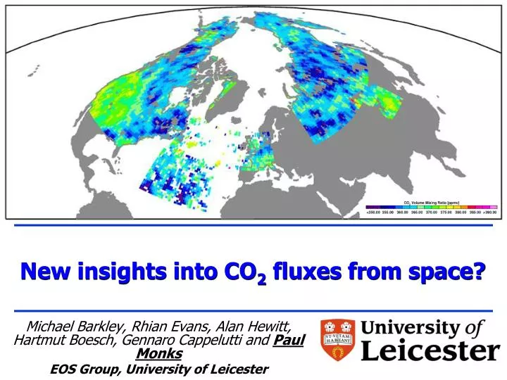
New insights into CO2 fluxes from space? Michael Barkley, Rhian Evans, Alan Hewitt, Hartmut Boesch, Gennaro Cappelutti and Paul Monks EOS Group, University of Leicester
The FSI algorithm: Overview • How do we measure atmospheric CO2? • WFM-DOAS retrieval technique (Buchwitz et al., JGR, 2000) designed to retrieve the total columns of CH4,CO, CO2, H2O and N2O from spectral measurements in NIR made by SCIAMACHY • Least squares fit of model spectrum + ‘weighting functions’ to observed sun-normalised radiance • We use WFM-DOAS to derive CO2 total columns from absorption at ~1.56 μm • Key difference to Buchwitz’s approach: • No look-up table • Calculate a reference spectrum for every single SCIAMACHY observation i.e. to obtain ‘best’ linearization point – no iterations • See “Measuring atmospheric CO2 using Full Spectral Initiation (FSI) WFM-DOAS” , Barkley et al., ACP, 6, 3517-3534,2006 • Computationally expensive SCIAMACHY SCIAMACHY, on ENVISAT, is a passive hyper-spectral grating spectrometer covering in 8 channels the spectral range 240-2040 nm at a resolution of 0.2-1.4 nm Typical pixel size = 60 x 30 km2
Cloud Filter SPICI (SRON) (Krijger et al, ACP, 2005) ‘A priori’ Data CO2 profiles taken from climatology (Remedios, ULeic) ECMWF: temperature, pressure and water vapour profiles ‘A priori’ albedo - inferred from SCIAMACHY radiance as a f(SZA) ‘A priori’ aerosol (maritime/rural/urban) SCIAMACHY Spectra, geolocation, viewing geometry, time Raw Spectra Process only if : cloud free, forward scan, SZA ‹75 SCIATRAN (Courtesy of IUP/IFE Bremen) LBL mode, HITRAN 2004 Calibration Non-linearity, dark current, ppg & etlaon I - Calibrated Spectra I0 – Frerick (ESA) Reference Spectrum + weighting functions (CO2, H2O and temperature) SCIAMACHY Spectrum (I/I0) WFM-DOAS fit CO2 Column (Normalise with ECMWF Surface Pressure) Accept only: Errors <5%, Range:340-400 ppmv Note: No scaling of FSI data
FSI Spectral fits • Good fit residuals • Retrievals errors: • Over land 1-4% • Over oceans 1-25%
North-South Gradients Mol Props Nov07
Validation Summary • FTIR • Park Falls ~ -2% • Egbert ~ -4% • TM3 • Bias ~ -2% • SCIAMACHY overestimates seasonal cycle by factor 2-3 with respect to the TM3 – reason? • Bias of TM3 w.r.t Egbert FTIR data ~ -2% • Aircraft– collocated observations in time & space • Sites over Siberia (r2 > 0.72-0.9) • Best at 1.5 km • Surface Sites - monthly averages • Time series comparisons (inc. aircraft) • Out of 17, 11 have r2 > 0.7
Can we learn anything? • Greater CO2 uptake by forests compared to crops & grass plains? • Identification of sub-continental CO2 sources/sinks ? Mol Props Nov07
ΔCO2 over target area CO2 mole fractions ending up into the release domain. These concentrations describe the overall CO2 collected by the air from the Earth's surface through its way to the release areas.
CO2 over target area absolute CO2 concentration of the release area + exchanged CO2 concentration = data comparable with those from satellite
Background CO2 (A) CO2 at release location is obtained from weighted background CO2 plus a weighted flux contribution. In simplified diagram, the thick arrow from direction C represents greatest surface contact time, and the greatest contribution of the background CO2. Land type A Release Location Land type B Land type C Background CO2 (C)
Land area is divided into a small grid. For each grid square the surface influence is multiplied by the strength of flux (from e.g. carbon tracker). Summing up all of the grid squares produces a delta CO2. Adding these to the weighted background, gives an atmospheric concentration, that is compared to the satellite. Strong absorber Compare to satellite Weak emitter Weak absorber
Monthly mean (left) + Standard Deviation (right) of CO2 fluxes from Carbon Tracker, over North America July 2003.
Surface influence (time spent at lowest altitude grid) of air released at 40-50N, 90-100W on 14th July 2003.
Retrieved FSI CO2 columns over North America on the 2nd July 2003.
Summary • Encouraging first results from the FSI algorithm • Good agreement with FT stations at Egbert & Park Falls (bias -2 to -4%) • Good agreement with TM3 model (more uptake in summer) • Good agreement with aircraft data over Siberia • Good agreement with AIRS CO2 (accounting for different vertical sensitivity) • Good agreement with surface network • Good correlation with vegetation spatial distribution • Key point: SCIAMACHY can track changes in near surface CO2 • Comparison of vegetation indices vs. CO2 indicate SCIAMACHY can track biological signal at regional level (though at limit of sensitivity) • Can we measure fluxes: • It is clear that there is information in the SCIAMACHY data on the biospheric fluxes • Preliminary estimates seem to show a quantitative correlation with carbon tracker when weighted for surface contact time • Further work is required and underway • Outlook - Very encouraging for GOSAT and OCO • ‘Measuring’ CO2 with a non-ideal instrument & ‘primitive’ algorithm Mol Props Nov07
Thanks also to… John Burrows and V. Rozanov IUP/IFE University of Bremen Alastair Manning and Claire Witham Met Office, UK AT2 Sep08
Flux datasets • Carbon Tracker: biosphere, sea, fossil fuel, fire and overall • JULES: vegetation (Joerg Kaduk, Geography, Leicester) • ECOSSE: soil (Jo Smith, Aberdeen) • NAEI: anthropogenic emissions JULES Gross Primary Production (GPP): rate at which an ecosystem produces, captures and stores chemical energy as biomass. Average over 5 years: 1999-2003. Units: kgC/m2/s.