Download
1 / 42
420 likes | 573 Views
Cloud parameters estimated by variational analysis of visible and infrared measurements from ATSR-2. Caroline Poulsen, Richard Siddans, Barry Latter and Brian Kerridge, Chris Mutlow, Sam Dean 2 , Don Grainger 2 , Gareth Thomas 2 , Graham Ewen 2 and Phil Watts 1

E N D
Cloud parameters estimated by variational analysis of visible and infrared measurements from ATSR-2 Caroline Poulsen, Richard Siddans, Barry Latter and Brian Kerridge, Chris Mutlow, Sam Dean2, Don Grainger2, Gareth Thomas2, Graham Ewen2 and Phil Watts1 Space Science and Technology Department Rutherford Appleton Laboratory UK Now at EUMETSAT Oxford University
Outline Why use ATSR? Why Variational Analysis? Forward Model Examples Validation Level 3 products Future
ATSR2/AATSR 0.55um 0.67um 0.87um 1.6um 3.7um 11um 12um ATSR Channels • Cloud Parameters Retrieved • Cloud top pressure/height • Cloud fraction • Cloud optical depth • Cloud effective radius • Cloud phase • Aerosol Parameters Retrieved • Aerosol optical depth • Aerosol effective radius • Auxillary information • ECMWF T and q profiles • MODIS surface albedo
Comparing measurements with calculations: Ice, water and mixed phase ice water
Basic principle is to maximise the accuracy the retrieved cloud parameters based on the measurements and any ‘apriori’ Allows us to characterise the error in each cloud parameter under the assumption of a reasonably plane parallel cloud model It’s a very flexible approach that enables us to utilise any prior information, for example on cloud fraction. All the clear sky atmospheric effects can be derived from NWP profiles. Allows us to utilise ALL the information in the measurements for each channel contributes to a greater or lesser extent to the retrieval of individual cloud parameters. Why use Optimal Estimation?
Plates Columns Rosettes Aggregates Ice clouds: complex particles Currently uses a combination of geometric optics (ray tracing); for large ice crystals and a T-matrix (ray tracing); method for small crystals.
Size distribution Water clouds: spherical drops Mie theory: solution of electromagnetic equations on dielectric sphere 10 mm drop, 0.87 mm wavelength Look up Tables Since real time calculations of cloud radiative properties are too slow calculations are made once DISORT (plane-parallel) model and incorporating rayleigh scattering and stored in easily accessible Look up Tables.
Tac(e.g. MODTRAN) Tbc Rs Cloud + Atmosphere/surface • Separate solar and ‘thermal’ models • Both embed cloud with precalculated radiative properties (LUTs) in clear atmosphere Solar model tre pc (f)
Atmosphere emitted Reflected Cloud emitted Transmitted Tac Rup Rdown B(T(pc))e Thermal model tre pc (f) Rbc From e.g. RTTOV
Guess a priori xo xb Calculate measurements y(xn) Compare J = [ym-y(xn)] Sy-1 [ym-y(xn)]T + [xn-xb] Sx-1 [xn-xb]T dx = - J’/J’’ (Newton’s Method) Adjust (minimise J) dJ < 0.1 or n>10 Stop! Inversion: Optimal estimation = 1D-Variational analysis. Same principles > 3D, 4D Var (assimilation)
Cost Function Compare J = [ym-y(xn)] Sy-1 [ym-y(xn)]T + [xn-xb] Sx-1 [xn-xb]T J = [ym-y(xn)] Sy-1 [ym-y(xn)]T Where ym are the radiances, Sy the measurement error covariance and y(xn) the cloud parameters modelled into radiance space. + [xn-xb] Sx-1 [xn-xb]T Where Xb is the apriori and Sx the apriori covariance.
Guess a priori xo xb Calculate measurements y(xn) Compare J = [ym-y(xn)] Sy-1 [ym-y(xn)]T + [xn-xb] Sx-1 [xn-xb]T dx = - J’/J’’ (Newton’s Method) Adjust (minimise J) dJ < 0.1 or n>10 Stop! Inversion: Optimal estimation = 1D-Variational analysis. Same principles > 3D, 4D Var (assimilation)
xsolution Minimising J: optically thick cloud -No a priori, -0.55, 1.6mmchannels - t, Re only xo
Retrieved Cloud Parameters Effective radius Fraction False colour Optical depth Cloud top pressure
Error Analysis and Quality Control False colour Error Cloud top pressure Cost Ssolution = J’’ solution = (Sx-1 + KT.Sy-1K)-1
Hercules - ERS-2 Coincidence Re validation against MRF FSSP probe Optical depth (scaled to fit) Effective radius ATSR FSSP
Validation at SGP 20th Oct. 1997 Microwave radiometer AATSR overpass17:26 SGP ARM data courtesy of Roger Marchand.
Case study 20th October 1997 LWP Effective radius Optical Depth
SGP validation Mean: -0.08 Stdev: 1.21 Optical depth calculated using Han et al J. Atmos Sci.,1995. Errors shown are the standard deviation of the matches used. Liquid water path is calculated using the technique of Frisch et al, J. Atmos Sci. 1995, the technique is only valid for non-raining, water clouds.
Validation of CTH Chilbolton 94GHz Galileo Radar
Comparison with ISCCP data ATSR-2 May 1999 Optical depth ISCCP Optical depth May 1999
Summary and plans • 6 years of ATSR-2 data processed at 3x3km resolution and a variety of level 3 products • Version 2 to begin soon with many improvements • Potential is there to use information from other satellites • Dual view tomographic cloud retrieval • Extension to AATSR- long time series • More validation, comparison with met. Office models
The ATSR cloud and aerosol algorithm was developed under funding from the following projects The end
Model adequate (J<1) Expected errors, S parameter dependent state dependent Information for assimilation (Discussed today Not discussed) Model inadequate (J>1) A priori out of range rogue values Measurements out of range calibration errors rogue values Model out of range multi-layer cloud shadows incorrect ice crystals incorrect surface reflectance incorrect statistical constraints QC: Summary
“Forward modelling”: Optical properties of average particle in ‘single scattering’ event Optical properties of a cloud of particles: multiple scattering Interaction of cloud radiative processes with atmosphere and surface y = y(x) “Inverse modelling”: x = ? (y) Guess cloud conditions (x) Calculate radiances y(x) Compare to measurements Change cloud conditions Retrieval (inversion): required steps Stop!
Hercules - ERS-2 Coincidence Re validation against MRF FSSP probe Optical depth (scaled to fit) Effective radius ATSR FSSP
Monthly Averaged Results May 1999 log10Optical depth May 1999 effective radius
Single particle Size distribution Water clouds: spherical drops Mie theory: solution of electromagnetic equations on dielectric sphere 10 mm drop, 0.87 mm wavelength