Download
1 / 25
250 likes | 384 Views
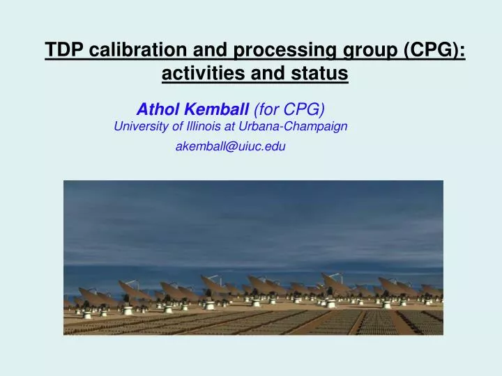
TDP calibration and processing group (CPG): activities and status. Athol Kemball (for CPG) University of Illinois at Urbana-Champaign akemball@uiuc.edu. Current CPG membership. Calgary. Athol Kemball (Illinois) ( Chair) Geoff Bower (UCB) Jim Cordes (Cornell; TDP PI ) Joe Lazio (NRL)

E N D
TDP calibration and processing group (CPG): activities and status Athol Kemball (for CPG) University of Illinois at Urbana-Champaign akemball@uiuc.edu
Current CPG membership . Calgary • Athol Kemball (Illinois) (Chair) • Geoff Bower (UCB) • Jim Cordes (Cornell; TDP PI) • Joe Lazio (NRL) • Colin Lonsdale (Haystack/MIT) • Steve Myers (NRAO) • Jeroen Stil (Calgary) • Greg Taylor (UNM) . . . Cornell . . MIT UIUC UCB . UNM NRL NRAO
Calibration and processing challenges for the SKA SKA-era telescopes & science require: • Surveys over large cosmic volumes (Ω,z), fine synoptic time-sampling Δt, and/or high completeness • High receptor count and data acquisition rates • Software/hardware boundary far closer to receptors than at present • Efficient, high-throughput survey operations modes Processing implications • High sensitivity, Ae/Tsys~104 m2K-1, wide-field imaging; • Demanding (t,ω,P) non-imaging analysis • Large O(109) survey catalogs High associated data rates (TBps), compute processing rates (PF), and PB/EB archives (LSST) (HI galaxy surveys, e.g. ALFALFA HI (Giovanelli et al. 2007); SKA requires a billion galaxy survey.)
SKA design & development phase (2007-2011) • Hardware design choices will define calibration and processing performance (e.g. dynamic range), cost, and feasibility. • In turn, need to identify calibration and processing constraints on hardware designs.
Calibration and processing design elements CPG goals • Determinefeasibilityof calibration and processing required to meet SKA science goals; • Determine quantitative cost equation contributions and design drivers as a function of key design parameters (e.g. antenna diameter, field-of-view, etc) • Measure algorithm cost and feasibility using prototype implementations • Demonstratecalibration and processing design elements using pathfinder data. US technology development emphases • Large-N small-diameter (LNSD) parabolic antenna design, wide-band single-pixel feeds, mid to high frequency range. • Close liaison with current international and national efforts. (ATA)
CPG immediate future steps November 2007 • 08/07: Initiate workplan development for CPG. Work ramps up. • 09/07: PrepSKA collaboration discussions. • 11/29/07: Face-to-face CPG meeting for in-depth workplan refinement. • 12/15/07: Finalize CPG project execution plan as part of general TDP project execution plan. • 01/08: URSI LNSD session. • 04/08: SKA CALIM conference Perth. • Q1-Q3/08: Hire CPG postdocs at UCB, MIT, & UIUC. • … Completed Completed Completed Completed 01/08 Completed Completed Completed In process
CPG activity timeline Oct 07 to present OCT NOV DEC JAN FEB MAR APR MAY JUN JUL OCT NOV CPG formation F2F planning meeting (Urbana) URSI 2008 LNSD session Project execution plan CPG meeting CPG F2F meeting (Perth) SKA CALIM 08 CPG F2F meeting (Washington DC) Execution plan implementation
CPG organization and coordination • Targeted design and development research working group, not production software development for SKA. • Prototype development will be software-package neutral, i.e any package allowing the research task can be used. • Close liaison with current international and national efforts. • Regular schedule of face-to-face meetings and telecons • All results aggregrated upwards into CPG Project Book; template defined. Intermediate results in memo series. • Internal mailing list, collaborative workspace, progress tracking wiki, and document repository. (Internal collaborative workspace: progress tracking and communication)
CPG engagement and partnerships • Community web-site launched to publicize intermediate results and activities • Engagement with: • National pathfinders (e.g. ATA, LWA, MWA, EVLA) • National center (NRAO) • Canadian efforts (Russ Taylor/Jeroen Sil [Calgary]) • International pathfinders: • MeerKAT • ASKAP • PrepSKA • Computer science & computer engineering groups (http://rai.ncsa.uiuc.edu/SKA/RAI_Projects_SKA_CPG.html)
CPG project execution plan CPG work breakdown structure • WBS 2.0: General • WBS 2.1: Signal transport • WBS 2.2: Calibration algorithms • WBS 2.3: Imaging, spectroscopy, & time-domain imaging • WBS 2.4: Scalability, & high-performance computing • WBS 2.5: RFI • WBS 2.6: Surveys • WBS 2.7: Data management Cross-cutting goals • LNSD feasibility: • e.g. dynamic range error budget • LNSD cost equation contributions (per calibration and processing technology)
Primary CPG deliverables • CPG work breakdown structure made up of prioritized calibration and processing technologies that are central to SKA LNSD design. • Key cross-cutting milestones are feasibility and cost assessments as envelope of design parameters (e.g. antenna diameter) and key science goals. • Feasibility and cost model release planned annually; successively refined based on research results.
Feasibility: imaging dynamic range Reference specifications (Schillizzi et al 2007) • Targeted λ20cm continuum field: 107:1. • Routine λ20cm continuum: 106:1. • Driven by need to achieve thermal noise limit (nJy) over plausible field integrations. • Spectral dynamic range: 105:1. • Current typical state of practice near λ ~ 20 cm given below. (de Bruyn and Brentjens, 2005) High-sensitivity deep fields Dynamic range
Image-plane calibration effect Visibility on baseline m-n Source brightness (I,Q,U,V) Direction on sky: ρ Feasibility: imaging dynamic range budget Basic imaging and equation for radio interferometry (e.g. Hamaker, Bregman, & Sault et al. 1996): Visibility-plane calibration effect Key contributions • Robust, high-fidelity image-plane (ρ) calibration: • Non-isoplanatism. • Antenna pointing errors. • Polarized beam response in (t,ω), … • Non-linearities, non-closing errors • Deconvolution and sky model representation limits • Dynamic range budget will be set by system design elements. (Bhatnagar et al. 2004; antenna pointing self-cal: 12µJy => 1µJy rms)
(Cornwell et al. 2006: example of 1.4 GHz edge effect at 2% PB level)
Feasibility: dynamic range assessment SKA dynamic range assessment – beyond the central pixel • Current achieved dynamic ranges degrade significantly with radial projected distance from field center, for reasons understood qualitatively (e.g. direction-dependent gains, sidelobe confusion etc.) • An SKA design with routine uniform, ultra-high dynamic range requires a quantitative dynamic range budget. • Strategies: • Real data from similar pathfinders (e.g. ATA, EVLA) are key. • Simulations are useful if relative dynamic range contributions or absolute fidelity are being assessed with simple models. • Newstatistical methods: • Assume convergent, regularized imaging estimator for brightness distribution within imaging equation; need to know sampling distribution of imaging estimator per pixel, but unknown PDF a priori: • Statistical resampling (Kemball & Martinsek 2005ff) and Bayesian methods (Sutton & Wandeldt 2005) offer new approaches.
MODEL-BASED BOOTSTRAP RESAMPLING EXAMPLE Np=1; Δt = 60 s Np=1; Δt = 150 s Monte Carlo reference variance image Np=1; Δt = 300 s Np=2; Δt = 900 s
WBS 2.3.1: Cost equation: wide-field image formation Algorithm technologies • 3-D transform (Perley 1999), facet-based tesselation / polyhedral imaging (Cornwell & Perley 1992), and w-projection (Cornwell et al. 2003). (Cornwell et al. 2003; facet-based vs w-projection algorithms)
WBS 2.3.1: Imaging cost equation contributions • LNSD data rates (Perley & Clark 2003): where D = dish diameter, B = max. baseline, Δν = bandwidth, and ν = frequency • Wide-field imaging cost ~ O(D-4 to -8) (Perley & Clark 2003; Cornwell 2004; Lonsdale et al 2004). • Full-field continuum imaging cost (derived from Cornwell 2004): • Strong dependence on 1/Dand B. Data rates of Tbps and computational costs in PF are readily obtained from underlying geometric terms. • Spectral line imaging costs exceed continuum imaging costs (further multiplier ) • Possible mitigation through FOV tailoring (Lonsdale et al 2004), beam-forming, and antenna aggregation approaches (Wright et al.) • 550 GBps/na2 (Lonsdale et al 2004) • Runaway petascale costs for SKA tightly coupled to design choices
WBS 2.4: Scalability Inconvenient truths • Moore’s Law holds, but high-performance architectures are evolving rapidly: • Breakpoint in clock speed evolution (2004) • Lateral expansion to multi-core processors and processor augmentation with accelerators • Theoretical performance ≠ actual performance • Sustained petascale calibration and imaging performance for SKA requires: • Demonstrated mapping of SKA calibration and imaging algorithms to modern HPC architectures, and proof of feasible scalability to petascale: [O(105) processor cores]. • Remains a considerable design unknown in both feasibility and cost. (Golap, Kemball et al. 2001, Coma cluster, VLA 74 MHz, parallelized facet-based wide-field imaging)
WBS 2.4: Scalability *Abe: Dell 1955 blade cluster – 2.33 GHz Intel Cloverton Quad-Core • 1,200 blades/9,600 cores • 89.5 TF; 9.6 TB RAM; 170 TB disk – Power/Cooling • 500 KW / 140 tons (Dunning 2007)
Commoditization effects in computing hardware costs models for general- purpose CPU and GPU accelerators at a fixed epoch (2007). Estimated from public data. WBS 2.4.5: Computing hardware cost models • Computing hardware system costs vary over key primary axes: • Time evolution (Moore’s Law) • Level of commoditization Moore’s Law for general-purpose Intel CPUs. Trend-line for Top 500 leading-edge performance.
WBS 2.4.5: Computing hardware cost models • Predicted leading-edge LINPACK Rmax performance from Top 500 trend-line (from data tyr = [1993, 2007]): • Cost per unit teraflop cTF(t), for a commiditzation factor η, Moore’s Law doubling time Δt, and construction lead time Δc: [with cTF(t0) = $300k/TF, t0 = 2007, η = [0.3-1.0], Δt ~ 1.5 yr, Δc ~ 1-4 yr]
WBS 2.4.5: Related computing cost components • Facility parameters: • One PF sustained requires tens MW; O(104) sq. ft. • Green innovations essential, will likely be mandatedin US by law: • Current US data centers 61bkWh • Will double by 2011; peak 12 GW, $7.4b per year electricity cost • Software development costs (Boehm et al. 1981): where β ~ ratio of academic to commerical software construction costs (~ 0.3-0.5); can mitigate through re-use (see adjacent) • LSST computing costs ~25% of project; order of magnitude smaller data rates than SKA (~ tens of TB per night). NCSA Petascale Computing Facility (20,000 ft2 machine room; chilled water with free cooling 6/12 months) (Kemball et al., 2007, “A component-based framework for radio-astronomical imaging software systems”, Software: Practice & Experience, 38 (5), 493-507)
CPG upcoming activities • CPG work plan continues per project execution plan. • Q2-Q3/08: Hire CPG postdocs at MIT, & UIUC. • 08/08: URSI GA 2008 (presentations and associated CPG meeting) • 10/08: First release of cost-feasibility LNSD model • …