Download
1 / 10
110 likes | 387 Views
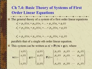
Ch 7.4: Basic Theory of Systems of First Order Linear Equations. The general theory of a system of n first order linear equations parallels that of a single n th order linear equation. This system can be written as x ' = P ( t ) x + g ( t ), where. Vector Solutions of an ODE System.

E N D
Ch 7.4: Basic Theory of Systems of First Order Linear Equations • The general theory of a system of n first order linear equations parallels that of a single nth order linear equation. • This system can be written as x' = P(t)x + g(t), where
Vector Solutions of an ODE System • A vector x = (t) is a solution of x' = P(t)x + g(t) if the components of x, satisfy the system of equations on I: < t < . • For comparison, recall that x' = P(t)x + g(t) represents our system of equations • Assuming P and g continuous on I, such a solution exists by Theorem 7.1.2.
Example 1 • Consider the homogeneous equation x' = P(t)x below, with the solutions x as indicated. • To see that x is a solution, substitute x into the equation and perform the indicated operations:
Homogeneous Case; Vector Function Notation • As in Chapters 3 and 4, we first examine the general homogeneous equation x' = P(t)x. • Also, the following notation for the vector functions x(1), x(2),…, x(k),… will be used:
Theorem 7.4.1 • If the vector functions x(1) and x(2) are solutions of the system x' = P(t)x, then the linear combination c1x(1) + c2x(2) is also a solution for any constants c1 and c2. • Note: By repeatedly applying the result of this theorem, it can be seen that every finite linear combination of solutions x(1), x(2),…, x(k) is itself a solution to x' = P(t)x.
Example 2 • Consider the homogeneous equation x' = P(t)x below, with the two solutions x(1) and x(2) as indicated. • Then x =c1x(1) + c2x(2) is also a solution:
Theorem 7.4.2 • If x(1), x(2),…, x(n) are linearly independent solutions of the system x' = P(t)x for each point in I: < t < , then each solution x = (t) can be expressed uniquely in the form • If solutions x(1),…, x(n) are linearly independent for each point in I: < t < , then they are fundamental solutions on I, and the general solution is given by
The Wronskian and Linear Independence • The proof of Thm 7.4.2 uses the fact that if x(1), x(2),…, x(n) are linearly independent on I, then detX(t) 0 on I, where • The Wronskian of x(1),…, x(n) is defined as W[x(1),…, x(n)](t) = detX(t). • It follows that W[x(1),…, x(n)](t) 0 on I iff x(1),…, x(n) are linearly independent for each point in I.
Theorem 7.4.3 • If x(1), x(2),…, x(n) are solutions of the system x' = P(t)x on I: < t < , then the Wronskian W[x(1),…, x(n)](t) is either identically zero on I or else is never zero on I. • This result enables us to determine whether a given set of solutions x(1), x(2),…, x(n) are fundamental solutions by evaluating W[x(1),…, x(n)](t) at any point t in < t < .
Theorem 7.4.4 • Let • Let x(1), x(2),…, x(n) be solutions of the system x' = P(t)x, < t < , that satisfy the initial conditions respectively, where t0 is any point in < t < . Then x(1), x(2),…, x(n) are fundamental solutions of x' = P(t)x.