Download
1 / 109
1.14k likes | 1.46k Views
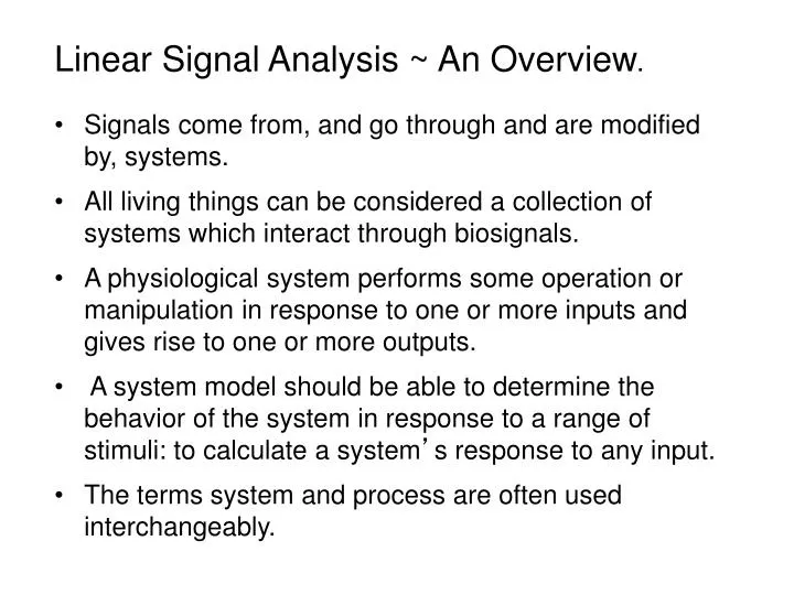
Linear Signal Analysis ~ An Overview. Signals come from, and go through and are modified by, systems. All living things can be considered a collection of systems which interact through biosignals.

E N D
Linear Signal Analysis ~ An Overview. • Signals come from, and go through and are modified by, systems. • All living things can be considered a collection of systems which interact through biosignals. • A physiological system performs some operation or manipulation in response to one or more inputs and gives rise to one or more outputs. • A system model should be able to determine the behavior of the system in response to a range of stimuli: to calculate a system’s response to any input. • The terms system and process are often used interchangeably.
Linear Time Invariant Systems • To predict the behavior of complex processes quantitatively in response to complex stimuli, severe simplifications and/or assumptions are invoked: • The process behaves in a linear manner. • Its basic characteristics do not change over time. • Combined, these two assumptions are referred to as a “linear time-invariant” (LTI) system. • A formal, mathematical definition of an LTI system is given in the next section, but the basic idea is intuitive: such systems exhibit proportionality of response (double the input/double the output) and they are stable over time.
Linear Systems Analysis • Assuming a system is LTI allows us to apply a powerful array of mathematical tools known collectively as “linear systems analysis.” • Living systems change over time, they are adaptive, and they are often nonlinear, but the power of linear systems analysis justifies the required assumptions or approximations. • Linearity can be approximated by using small-signal conditions since, when a range of action is restricted, many systems behave more-or-less linearly. • Alternatively, piecewise linear approaches can be used where the analysis is confined to operating ranges over which the system behaves linearly.
Linear Systems Analysis (cont) • A feature of linear systems is that they can be represented solely by linear differential equations. • Any linear system, no matter how complex, can be represented by combinations of at most four element types: arithmetic (addition and subtraction), scaling (i.e., multiplication by a constant), differentiation, and integration. • A typical system might consist of only one of these four basic elements, but usually are made up of a combination of basic operators. • A summary of these basic elements types is provided later in this section.
Analog and System Representations of Linear Processes • Either analog or systems models can be used to represent linear processes. • The primary difference between analog and systems models is the way the underlying processes are represented. • In analog analysis, individual components are represented by analogous elements while the component of a systems model is an input-output process. • Arithmetic operations are determined by the way the elements are arranged in the model so that only three elements - scaling, differentiation, and integration - are needed.
Analog Model Example This simple electric circuit is actually an analog model of the cardiovascular system known as the “windkessel model.” In this circuit, voltage represents blood pressure, current represents blood flow, RP and CP are the resistance and compliance of the systemic arterial tree, and Zo is the characteristic impedance of the proximal aorta. Circuit models are covered in Chapters 10 and 11; we find that using an electrical network to represent what is basically a mechanical system is mathematically appropriate.
System Model Example A model of the neural pathways that mediate the vergence eye movement response, the processes used to turn the eyes inward to track visual targets at different depths, is shown. The model shows three different neural paths converging on the elements representing the oculomotor plant (the right-most system element).
Analog versus System Models • Systems models and concepts are very flexible: inputs can take many different energy forms (chemical, electrical, mechanical, or thermal), and outputs can be of the same or different energy forms. • System representations can be more succinct. • Elements in analog models relate more closely to the underlying physiological processes, system representations provide a better overall view of the system under study. • The next few chapters address system models while Chapters 10 and 11 are devoted to analog models and circuits.
Linear Elements ~ Linearity, Time Invariance, Causality All linear systems are composed of linear elements. The concept of linearity has a rigorous definition, but the basic concept is one of proportionality of response: if you double the stimulus into a linear system, you get twice the response. Stating this proportionality property mathematically: if the independent variables of linear function are multiplied by a constant, k, the output of the function is simply multiplied by k. Assuming:
Linear Properties If f is a linear function: In addition, if: y = f(x) and ; then: Similarly if: y = f(x) and ; then: Derivation and integration are linear operations. When they are applied to linear functions, these operations preserve linearity.
Time Invariance If the system has the same behavior at any given time; that is, its basic response characteristics do not change over time, it is said to be time-invariant. Time invariance could be thought of as a stricter version of stationarity since a time invariant system would also be stationary. The mathematical definition of a time invariant function, f, is given as: Systems that are both linear and time-invariant are referred to as “linear time-invariant” systems, usually abbreviated as “LTI” systems.
Causality and Memory • If a system responds only to current and past inputs, the system is termed “causal.” • Real-world systems are causal, but if a system is represented in a computer it could be made to produce an output that, for any given time period, depends on futures values of a signal. • If a system only responds to its current input and not to inputs past, it is said to be “memoryless.” • Conversely, a system whose current output depends to some extend on past inputs, it is said to possess “memory.”
Superposition • Superposition states that when two or more influences act on a process, the result is the same as the summation of the process’s response to each influence acting alone. • The principle of superposition means that when two or more inputs are active in a system, a solution can be obtained by solving the problem as if each source was acting alone, then algebraically summing these partial solutions. • The sources could be anywhere in the system. • In system representations, the multiple sources are usually at one location, a location defined as the input.
Solutions Using Frequency Domain Decomposition • In system models, ‘multiple sources’ could be just the sinusoidal components of a single more complicated input signal. • If superposition holds, then the response of any LTI system can be found to any input by: • decomposing the signal into its sinusoidal components using the Fourier series or Fourier transform; • finding the system’s response to each sinusoid in the decomposition; • summing the individual sinusoidal responses using the Fourier series equation.
Solutions Using Frequency Domain Decomposition (cont) • This decomposition strategy may seem like a lot of work were it not for the fact that step 2, finding the response of any linear system to a sinusoidal input, can be accomplished using only algebra. • Even for systems that contain calculus operations like integration or differentiation, techniques exist that convert these operations to algebraic operation. • This strategy, combining frequency decomposition with the ease of algebraic solutions, motivates many of the concepts developed in the next few chapters.
Solutions Using Time Domain Segmentation • You can also determine the response of a linear system in the time domain by decomposing the signal using standard calculus tricks: • divide the signal into infinitely small segments; • find the response of the system to each small time segment; • sum the segment responses. • This is just a time domain analogy to the frequency domain strategy described in the last paragraph. It is developed in Chapter 7.
Systems Analysis and Systems Models • Systems models usually represent processes using so-called “black box” components. • Each element of a systems model consists only of a mathematically defined input-output relationship and is represented by a geometrical shape, usually a rectangle. • No effort is made to determine what is actually inside the box, hence the term black box: only the element’s relationship between input and output is of importance.
System Elements A typical element in a systems element (or entire system) is shown graphically as a box, or sometimes as a circle when an arithmetic process is involved. Two such elements are shown. The inputs and outputs of all elements are signals with a well-defined direction of flow or influence. These signals and their direction of influence are shown by lines and arrows connecting the system elements.
Transfer Function The letter G in this element represents the mathematical description of the element: the mathematical operation that converts the input signal into an output signal. Stated mathematically: Output = G(Input) The variable G is general and could be any linear relationship, and the terms Input and Output could represent a variety of signal modalities of varying complexity. Rearranging this basic equation, G can be expressed as the ratio of output to input: Because it relates the Output to the Input of a system, this equation is called the “transfer function.”
Transfer Function (cont) • The transfer function is a critical concept in linear systems analysis because it defines the input/output relationship of a system, the only concern in a classical system model. • Although the transfer function concept is sometimes used very generally, in the context of linear systems analysis it is an algebraic multiplying function. • Linear system elements can be represented algebraically which leads to a transfer function that is algebraic. • The overall input/output relationship can be determined from the input/output relationships of each element using algebra.
Transfer Function Algebra The transfer function is an algebraic multiplier. When two systems are connected in series the transfer function of the overall paired systems is just the product of the two individual transfer functions: Out2 = G2 x In2 and Out1 ≡ In2 = G1 x In1, then: Out2 = G2 x (G1 x In1) = G2 G1 In1. and the overall transfer function for the 2 series elements is:
Multiple Transfer Functions Note that the overall transfer function of the combined systems in Figure 5.4 would be the same even if the order of the two systems was reversed. This is a property termed “associativity.” We can extend this concept to any number of system elements in series: The overall transfer function is just the product of the individual series element transfer functions: In practice, determining the transfer function of most biological systems is challenging and usually involves extensive empirical observation of the input/output relationship.
Example 5.1Find the transfer function for the systems model shown. The mathematical description of each element is either an algebraic term or an arithmetic operation, in this case subtraction. G and H are assumed to be linear algebraic functions, so they produce an output that is the product of function times the input. The system shown is a classic feedback system because the output is coupled to the input via the lower pathway Feedfoward Pathway Feedback Pathway G is called the “feedforward gain” H is called the “feedback gain.”
Example 5.1 Solution Generate an algebraic equation based on the configuration and the transfer equation of each element: Output = G x Input).
Example 5.1 Analysis Analysis: The solution found in this problem is known as the “feedback equation:” This equation will be used in later analyses of more complex systems. In this example, G and H can be anything as long as they can be treated algebraically. When the individual elements contain differential or integral operations in their input/output relationships, special techniques are used to change calculus operations into algebraic manipulations. This equation and the general strategy to find this equation applies even when the system contains more complicated elements.
Example 5.2 There is a MATLAB function on the disk that represents a system. The function is called process_x and it takes an input signal, x, and generates an output signal y (as in: y = process(x) ) We are to determine if process_x is a linear process over the range of 0 to ±100 signal units. We can input to the process any signal we desire and examine the output. Input Output Unknown Process
Example 5.2 Solution: The basic strategy is to input a number of signals with different amplitudes and determine if the outputs are proportional. What is the best signal to use? The easiest might be to input a number of constant signals, e.g., x = ±1, ±10, ±100 …, The output should be proportional. If the process contains a derivative or integral operation (both are linear operations), a constant input would be hard to interpret. (The output of a derivative element to any constant is zero.) A sinusoid would be ideal because the derivative or integral of a sinusoid is still a sinusoid, and only the amplitude and phase would be different.
% Example 5.2 Example to evaluate and unknown process is linear. % t = 0:2*pi/500:2*pi; % Sine wave time function, 500 points for k = 1:100 % Amplitudes (k) will vary from 1 to 100 x = k*sin(t); % Generate a 1 cycle sine wave y = process_x(x); % Input sine to process output(k) = max(y); % Save max value of output end plot(output); % Horizontal axis will be max. amplitude …….label axes……. Analysis: The first instruction generates the time vector. A ‘for-loop’ is used to generate sine waves with amplitudes ranging from ±1 to ±100. Each sine wave is an input signal to process_x. The function process_x produces an output signal, y, and the peak value of the output is plotted.
Example 5.2 Results Output The output to a sine wave input is sinusoidal, but the amplitude and phase are modified. Input The plot of sinusiodal output amplitudes is a straight line indicating the process_x is a linear process, at least of the range of amplitudes tested. Deriving the exact input/output equation for an unknown process using external signals is known as “system identification.”
Analog Analysis: Summary • Analog models represent the physiological process using elements that are, to some degree, analogous to those in the physiological process. • Good analog models can represent the system at a lower level, and in greater detail, than systems models. • Analog models provide better representation of secondary features such as energy use, which is usually similar between analog elements and the real-world components these elements represent. • In analog models, the interaction between components may not be obvious from inspection of the model. • .
System Analysis: Summary • System models emphasize component interaction, particularly with regard to information flow, and clearly show the overall organization. • Influence between elements is explicitly shown by lines with arrows. • This can greatly clarify the control structure of a complex system. • The most significant advantage of the systems approach is what it does not represent: • It allows the behaviors of biological processors to be described quantitatively without requiring details of the underlying physiological mechanism.
The Response of System Elements to Sinusoidal Inputs: Phasor Analysis • If the signals or variables in a system are sinusoidal or can be converted to sinusoids using the Fourier series or Fourier transform, then a technique known as phasor analysis can be used to convert calculus operations into algebraic operations. • Phasor analysis combines complex representation of sinusoids with the fact that calculus operations (integration and differentiation) change only the magnitude and phase of a sinusoid. • This analysis assumes the signals are in sinusoidal steady-state.
Calculus Operations on Sinusoids • The frequency and basic shape of a sinusoid is not modified by calculus operations or scaling or arithmetic operations. • Linear elements will not alter the frequency and shape of a sinusoid. • That means that in a linear system, if the input is a sinusoidal steady-state signal, then all system variables including the output will be sinusoidal • All signals in such an LTI system can be described by the same general equation: • x(t) = A cos(ωt + θ) = A cos(2πft + θ) • where the values of A and θ can be modified by the system elements, but the value of ω (or f) will be the same throughout the system.
Quantitative Features of a Sinusoid • Sinusoids require just three variables for complete description: amplitude, phase and frequency. • If the frequency is always the same, as it would be for any variable of an LTI system, then we really only need to keep track of two variables: amplitude and phase. • This suggests that complex variables and complex arithmetic can simplify the mathematics of sinusoids, since a single complex variable is actually two (independent) variables rolled into one (i.e., a + jb). • A single complex number or variable should be able to describe the amplitude and phase of a sinusoid.
Complex Representation of a Sinusoid To find a way to represent a sinusoid by a single complex variable, we return to the complex representation of sinusoids given by Euler’s equation: or in terms of the general equation for a sinusoid: Comparing the basic sinusoid equation with the equation above shows that only the real part of ejx is needed to represent a sinusoid
Complex Representation of a Sinusoid (cont) If all variables in an equation contain the real part of the complex sinusoid, the real terms can be dropped, since if: In general, if Re A = Re B, A does not necessarily equal B. However the only way the Re Aejωt can equal theRe Bejωt at all values of t is if A = B. Since all variables in a sinusoidally-driven LTI will contain the ‘Re’ operator, these terms can be removed from the equations as was done in the equation above. They do not actually cancel; they are just unnecessary since the equality stands just as well without them.
Phase Representation of a Sinusoid Similarly, since all variables will be at the same frequency, the identical ejωt term will appear in each variable and will cancel after the Re’s are dropped. Therefore, a general sinusoid of can be represented by a single complex number: where Aejθ is the “phasor” representation of a sinusoid The phasor is not the same as a sinusoid mathematically, but a transformation to a complex exponential representation without loss of information. In the phasor representation, the frequency, ω, is not explicitly stated, but is understood to be associated with every variable in the system.
Phasor Calculus: the Derivative To determine the derivative of the phasor representation of a sinusoid, begin with the original complex definition of a sinusoid (i.e. Re Aejθejωt): The derivative of a phasor is the just the original phasor, but multiplied by jω. Hence, in phasor representation, taking the derivative is accomplished by multiplying the original term by jω, and a calculus operation has been reduced to a simple arithmetic operation:
Phasor Calculus: the Integral Integration can be performed in the phasor domain simply by dividing by jω: and the operation of integration becomes an arithmetic operation: Since 1/j is shown in the text to be the same as -j, the integral operation can also be described as:
Phasor Arithmetic: Multiplying by j Multiplying by j in complex arithmetic is the same as shifting the phase by 90 degrees, which follows directly from Euler’s equation: Substituting in cos(x + 90) for – sin x, and sin(x + 90) for cos x, je jx becomes: This is the same as e jx+90which equals e jx e 90 je jx = ejxe90
Phasor Arithmetic: Dividing by j Dividing by j is the equivalent of shifting the phase by - 90 deg: Substituting in cos(x – 90) for sin x, and sin(x – 90) for -cos x; becomes Phasors turn calculus operations into algebraic operations as long as we have sinusoidal steady-state signals.
Example 5.3Find the derivative of x(t) = 10 cos(2t + 20) using phasor analysis. Solution: Convert x(t) to phasor representation (represented as x(jω)), multiply by jω, then take the inverse phasor transform: Since cos(x) = sin(x + 90) = -sin(x - 90), this can also be written as -20 sin(2t + 20), which is obtained from straight differentiation.
Phasor Notation • A shorthand notation is common for the phasor description of a sinusoid. Rather than write Vejθ, we simply write V θ (stated as V and at an angle of θ). • Capital letters are usually used for the variable. • Frequency is in radians/sec, ω, rather than in Hz. • Hence, the time-phasor transformation for variable v(t) can be stated as: v(t) V(ω) = V θ For example, the phasor representation of 20 cos (2t + 110) would be written as 20 110.
The Transfer Function • The transfer function introduced previously gets its name because it describes how an input, Input(ω), is ‘transferred’ to the output, Output(ω). • Theconcept of the transfer function is so compelling that it has been generalized to include many different types of processes or systems with different types of inputs and outputs. • In the phasor domain, the transfer function is a modification of the original equation:
Example 5.4Find the transfer function, PA(ω)/FIN(ω), for the linearized model of the Guyton-Coleman body fluid balance system using phasor analysis. This model describes how the arterial blood pressure PA in mmHg responds to a small change in fluid intake, FIN in ml/min. Solution: The two elements in the upper path can be combined into a single element and the feedback equation applied.
Example 5.4 Result The transfer function of the combined element is just the product of the two individual transfer functions: The resulting system has the same configuration as the feedback system which has already been solved in Example 5.1 Substituting the expressions for G and H into the feedback equation gives the transfer function of this system:
Example 5.4 Analysis: This transfer function applies to any input signal at any frequency, ω, as long as it is ‘sinusoidal steady-state.’ Note that the denominator consists of a real and an imaginary part, and that the constant term is normalized to 1.0. This is the common format for transfer function equations: the lowest power of ω, usually a constant term, is normalized to 1.0. Systems having transfer functions with a 1+ jkω term in the denominator, where k is a constant, are called “first-order” systems. The output of this system to a specific sinusoidal input is determined in the next example.
Example 5.5 Find the output of the system in the last example if the input signal is FIN(t) = 0.5 sin(0.3t + 20) ml/min. Note that time has been scaled to hours even though the input is in ml/min. Solution: Since phasors are based on cosines, we first need to convert FIN(t) to a cosine wave. sin(ωt) = cos(ωt - 90), so FIN(t) = 0.5 cos(0.3t – 70) ml/min. In phasor notation the input signal is: FIN(t) = 0.5 cos(0.1t – 70) FIN(ω) = 0.570 ml/min From the solution to Example 5.4, the transfer function is:
Example 5.5 Solution (cont) Solving for Out(ω) and then substituting in 0.5 -70 for In(ω) and letting ω = 0.3: The rest of the problem is just working out the complex arithmetic. To perform division (or multiplication), it is easiest to have a complex number in polar form. The denominator becomes: Substituting and solving: Converting to the time domain: PA(t) = 1.64 cos(0.3t -150) mmHg
Example 5.5 Analysis So the arterial pressure response to this input is a sinusoidal variation in blood pressure of 4.48 mmHg. ERROR – should be 1.64 That variation has a phase of 150 deg, which is shifted 80 deg from the input phase. The corresponding time delay between the stimulus and response sinusoid can be found from Eq. 2.7: So the response is delayed 4.65 hrs from the stimulus due to the long delays in transferring fluid into the blood. AND “out of the blood.” As with many physiological systems, generating a sinusoidal stimulus, in this case a sinusoidal variation in fluid intake, is challenging. Remember the INSENSATE Losses!!!