Download
1 / 36
360 likes | 490 Views
Yang-Mills ground-state wavefunctional in 2+1 dimensions. (in collaboration with Jeff Greensite) J. Greensite, ŠO, Phys. Rev. D 77 (2008) 065003, arXiv:0707.2860 [hep-lat]. Motivation.

E N D
Yang-Mills ground-state wavefunctional in 2+1 dimensions (in collaboration with Jeff Greensite) J. Greensite, ŠO, Phys. Rev. D 77 (2008) 065003, arXiv:0707.2860 [hep-lat] Seminar, Institut f. Physik, Karl-Franzens-Universität, Graz
Motivation • “QCD field theory with six flavors of quarks with three colors, each representedby a Dirac spinor of four components, and with eightfour-vector gluons, is aquantum theory of amplitudes for configurations each of which is 104 numbers ateach point in space and time. To visualize all this qualitatively is too difficult. Thething to do is to take some qualitative feature to try to explain, and then to simplifythe real situation as much as possible by replacing it by a model which is likely tohave the same qualitative feature for analogous physical reasons. • The feature we try to understand is confinement of quarks. • We simplify the model in a number of ways. • First, we change from three to twocolors as the number of colors does not seem to be essential. • Next we suppose there are no quarks. Our problem of the confinement of quarkswhen there are no dynamic quarks can be converted, as Wilson has argued, to a question of the expectation of a loop integral. Or again even with no quarks,there is a confinement problem, namely the confinement of gluons. • The next simplification may be more serious. We go from the 3+1 dimensions ofthe real world to 2+1. There is no good reason to think understanding what goeson in 2+1 can immediately be carried by analogy to 3+1, nor even that the twocases behave similarly at all. There is a serious risk that in working in 2+1dimensions you are wasting your time, or even that you are getting false impressionsof how things work in 3+1. Nevertheless, the ease of visualization is so much greaterthat I think it worth the risk. So, unfortunately, we describe thesituation in 2+1 dimensions, and we shall have to leave it to future work to see whatcan be carried over to 3+1.” Seminar, Institut f. Physik, Karl-Franzens-Universität, Graz
Seminar, Institut f. Physik, Karl-Franzens-Universität, Graz
Introduction • Confinement is the property of the vacuum of quantized non-abelian gauge theories. In the hamiltonian formulation in D=d+1 dimensions and temporal gauge: Seminar, Institut f. Physik, Karl-Franzens-Universität, Graz
At large distance scales one expects: • Halpern (1979), Greensite (1979) • Greensite, Iwasaki (1989) • Kawamura, Maeda, Sakamoto (1997) • Karabali, Kim, Nair (1998) • Property of dimensional reduction: Computation of a spacelike loop in d+1 dimensions reduces to the calculation of a Wilson loop in Yang-Mills theory in d Euclidean dimensions. Seminar, Institut f. Physik, Karl-Franzens-Universität, Graz
Suggestion for an approximate vacuum wavefunctional Seminar, Institut f. Physik, Karl-Franzens-Universität, Graz
Warm-up example: Abelian ED Seminar, Institut f. Physik, Karl-Franzens-Universität, Graz
Seminar, Institut f. Physik, Karl-Franzens-Universität, Graz
Free-field limit (g!0) Seminar, Institut f. Physik, Karl-Franzens-Universität, Graz
Zero-mode, strong-field limit (D=2+1) • D. Diakonov (private communication to JG) • Let’s assume we keep only the zero-mode of the A-field, i.e. fields constant in space, varying in time. The lagrangian is and the hamiltonian operator • Natural choice - 1/V expansion: Seminar, Institut f. Physik, Karl-Franzens-Universität, Graz
Keeping the leading term in V only: • The equation is solved by: since Seminar, Institut f. Physik, Karl-Franzens-Universität, Graz
Now the proposed vacuum state coincides with this solution in the strong-field limit, assuming • The covariant laplacian is then • Let’s choose color axes so that both color vectors lie in, say, (12)-plane: Seminar, Institut f. Physik, Karl-Franzens-Universität, Graz
The eigenvalues of M are obtained from • Our wavefunctional becomes • In the strong-field limit Seminar, Institut f. Physik, Karl-Franzens-Universität, Graz
D=3+1 Seminar, Institut f. Physik, Karl-Franzens-Universität, Graz
Seminar, Institut f. Physik, Karl-Franzens-Universität, Graz
Dimensional reduction and confinement • What about confinement with such a vacuum state? • Define “slow” and “fast” components using a mode-number cutoff: • Then: Seminar, Institut f. Physik, Karl-Franzens-Universität, Graz
Effectively for “slow” components we then get the probability distribution of a 2D YM theory and can compute the string tension analytically (in lattice units): • Non-zero value of m implies non-zero string tension and confinement! • Let’s revert the logic: to get with the right scaling behavior ~ 1/2, we need to choose Seminar, Institut f. Physik, Karl-Franzens-Universität, Graz
Why m02 = -0 + m2 ? • Samuel (1997) Seminar, Institut f. Physik, Karl-Franzens-Universität, Graz
Non-zero m is energetically preferred • Take m as a variational parameter and minimize <H > with respect to m: • Assuming the variation of K with A in the neighborhood of thermalized configurations is small, and neglecting therefore functional derivatives of K w.r.t. A one gets: Seminar, Institut f. Physik, Karl-Franzens-Universität, Graz
Abelian free-field limit: minimum at m2 = 0 → 0. Seminar, Institut f. Physik, Karl-Franzens-Universität, Graz
Non-abelian case: Minimum at non-zero m2 (~ 0.3), though a higher value (~ 0.5) would be required to get the right string tension. • Could (and should) be improved! Seminar, Institut f. Physik, Karl-Franzens-Universität, Graz
Calculation of the mass gap • To extract the mass gap, one would like to compute in the probability distribution: • Looks hopeless, K[A] is highly non-local, not even known for arbitrary fields. • But if - after choosing a gauge - K[A] does not vary a lot among thermalized configurations … then something can be done. • Numerical simulation Seminar, Institut f. Physik, Karl-Franzens-Universität, Graz
Numerical simulation of |0|2 • Define: • Hypothesis: • Iterative procedure: Seminar, Institut f. Physik, Karl-Franzens-Universität, Graz
Practical implementation: choose e.g. axial A1=0 gauge, change variables from A2 to B. Then Spiral gauge • given A2, set A2’=A2, • the probabilityP[A;K[A’]] is gaussian in B, diagonalize K[A’] and generate new B-field (set of Bs) stochastically; • from B, calculate A2 in axial gauge, and compute everything of interest; • go back to the first step, repeat as many times as necessary. • All this is done on a lattice. • Of interest: • Eigenspectrum of the adjoint covariant laplacian. • Connected field-strength correlator, to get the mass gap: • For comparison the same computed on 2D slices of 3D lattices generated by Monte Carlo. Seminar, Institut f. Physik, Karl-Franzens-Universität, Graz
Eigenspectrum of the adjoint covariant laplacian Seminar, Institut f. Physik, Karl-Franzens-Universität, Graz
Mass gap Seminar, Institut f. Physik, Karl-Franzens-Universität, Graz
Seminar, Institut f. Physik, Karl-Franzens-Universität, Graz
Summary (of apparent pros) • Our simple approximate form of the confining YM vacuum wavefunctional in 2+1 dimensions has the following properties: • It is a solution of the YM Schrödinger equation in the weak-coupling limit … • … and also in the zero-mode, strong-field limit. • Dimensional reduction works: There is confinement (non-zero string tension) if the free mass parameter m is larger than 0. • m > 0 seems energetically preferred. • If the free parameter m is adjusted to give the correct string tension at the given coupling, then the correct value of the mass gap is also obtained. Seminar, Institut f. Physik, Karl-Franzens-Universität, Graz
Open questions (or contras?) • Can one improve (systematically) our vacuum wavefunctional Ansatz? • Can one make a more reliable variational estimate of m? • Comparison to other proposals? • Karabali, Kim, Nair (1998) • Leigh, Minic, Yelnikov (2007) • What about N-ality? • Knowing the (approximate) ground state, can one construct an (approximate) flux-tube state, estimate its energy as a function of separation, and get the right value of the string tension? • How to go to 3+1 dimensions? • Much more challenging (Bianchi identity, numerical treatment very CPU time consuming). • The zero-mode, strong-field limit argument valid (in certain approximation) also in D=3+1. Comparison to KKN N-ality Flux-tube state Seminar, Institut f. Physik, Karl-Franzens-Universität, Graz
Elements of the KKN approach • Matrix parametrisation: • Jakobian of the transformation leads to appearance of a WZW-like term in the action. Seminar, Institut f. Physik, Karl-Franzens-Universität, Graz
Comparison to KKN • Wavefunctional expressed in terms of still another variable: • It’s argued that the part bilinear in field variables has the form: • The KKN string tension following from the above differs from string tensions obtained by standard MC methods, and the disagreement worsens with increasing . Seminar, Institut f. Physik, Karl-Franzens-Universität, Graz
N-ality • Dimensional reduction form at large distances implies area law for large Wilson loops, but also Casimir scaling of higher-representation Wilson loops. • How does Casimir scaling turn into N-ality dependence, how does color screening enter the game? • A possibility: Necessity to introduce additional term(s), e.g. a gauge-invariant mass term • Cornwall (2007) … but color screening may be contained! • Strong-coupling: • Greensite (1980) Seminar, Institut f. Physik, Karl-Franzens-Universität, Graz
Guo, Chen, Li (1994) Seminar, Institut f. Physik, Karl-Franzens-Universität, Graz
Seminar, Institut f. Physik, Karl-Franzens-Universität, Graz
Flux-tube state • A variational trial state: • The energy of such a state for a given quark-antiquark separation can be computed from: • On a lattice: • Work in progress. Seminar, Institut f. Physik, Karl-Franzens-Universität, Graz
Epilogue/Apologies “It is normal for the true physicist not to worry toomuch about mathematical rigor. And why? Because onewill have a test at the end of the day which is the confrontationwith experiment. This does not mean that sloppinessis admissible: an experimentalist once told me thatthey check their computations ten times more than thetheoreticians! However it’s normal not to be too formalist.This goes with a certain attitude of physicists towardsmathematics: loosely speaking, they treat mathematics asa kind of prostitute. They use it in an absolutely free andshameless manner, taking any subject or part of a subject,without having the attitude of the mathematician whowill only use something after some real understanding.” • Alain Connes in an interview with C. Goldstein and G. Skandalis, EMS Newsletter, March 2008. Seminar, Institut f. Physik, Karl-Franzens-Universität, Graz