Download
1 / 22
240 likes | 388 Views
Ground-state solution of the Yang –Mills Schrödinger equation in 2+1 dimensions. (in collaboration with Jeff Greensite , SFSU) J. Greensite, ŠO, Phys. Rev. D 77 (2008) 065003, arXiv:0707.2860 [hep-lat]. A few quotes plus a bit of philately.

E N D
Ground-state solution of the Yang–Mills Schrödinger equation in 2+1 dimensions (in collaboration with Jeff Greensite, SFSU) J. Greensite, ŠO, Phys. Rev. D 77 (2008) 065003, arXiv:0707.2860 [hep-lat] Erwin Schrödinger Symposium 2009, Prague
A few quotes plus a bit of philately • “The mathematical framework of quantum theory has passed countless successful tests and is now universally accepted as a consistent and accurate description of all atomic phenomena.” [Erwin Schrödinger (?)] Erwin Schrödinger Symposium 2009, Prague
“QCD field theory with six flavors of quarks with three colors, each representedby a Dirac spinor of four components, and with eightfour-vector gluons, is aquantum theory of amplitudes for configurations each of which is 104 numbers ateach point in space and time. To visualize all this qualitatively is too difficult. Thething to do is to take some qualitative feature to try to explain, and then to simplifythe real situation as much as possible by replacing it by a model which is likely tohave the same qualitative feature for analogous physical reasons. • The feature we try to understand is confinement of quarks. • We simplify the model in a number of ways. • First, we change from three to twocolors as the number of colors does not seem to be essential. • Next we suppose there are no quarks. Our problem of the confinement of quarkswhen there are no dynamic quarks can be converted, as Wilson has argued, to a question of the expectation of a loop integral. Or again even with no quarks,there is a confinement problem, namely the confinement of gluons. […] • The next simplification may be more serious. We go from the 3+1 dimensions ofthe real world to 2+1. There is no good reason to think understanding what goeson in 2+1 can immediately be carried by analogy to 3+1, nor even that the twocases behave similarly at all. There is a serious risk that in working in 2+1dimensions you are wasting your time, or even that you are getting false impressionsof how things work in 3+1. Nevertheless, the ease of visualization is so much greaterthat I think it worth the risk. So, unfortunately, we describe thesituation in 2+1 dimensions, and we shall have to leave it to future work to see whatcan be carried over to 3+1.” [Richard P. Feynman (1981)] Erwin Schrödinger Symposium 2009, Prague
SLOVENSKO 1 € fyzik Erwin Schrödinger Symposium 2009, Prague
Introduction • Confinement is the property of the vacuum of quantized non-abelian gauge theories. In the hamiltonian formulation in D=d+1 dimensions and temporal gauge: Erwin Schrödinger Symposium 2009, Prague
At large distance scales one expects: • Halpern (1979), Greensite (1979) • Greensite, Iwasaki (1989) • Kawamura, Maeda, Sakamoto (1997) • Karabali, Kim, Nair (1998) • Property of dimensional reduction: Computation of a spacelike Wilson (-Wegner) loop in d+1 dimensions reduces to the calculation of a loop in Yang-Mills theory in d Euclidean dimensions. Erwin Schrödinger Symposium 2009, Prague
Suggestion for an approximate vacuum wavefunctional “It is normal for the true physicist not to worry toomuch about mathematical rigor. […]This goes with a certain attitude of physicists towardsmathematics: loosely speaking, they treat mathematics asa kind of prostitute. They use it in an absolutely free andshameless manner, taking any subject or part of a subject,without having the attitude of the mathematician whowill only use something after some real understanding.” (Alain Connes, interview with C. Goldstein and G. Skandalis, EMS Newsletter, 03/2008) Erwin Schrödinger Symposium 2009, Prague
Warm-up example: Abelian ED Erwin Schrödinger Symposium 2009, Prague
Free-field limit (g!0) Erwin Schrödinger Symposium 2009, Prague
Zero-mode, strong-field limit • D. Diakonov (private communication) • Let’s assume we keep only the zero-mode of the A-field, i.e. fields constant in space, varying in time. The lagrangian is and the hamiltonian operator • Solution (up to 1/V corrections): Erwin Schrödinger Symposium 2009, Prague
Now the proposed vacuum state coincides with this solution in the strong-field limit, assuming • The covariant laplacian is then • In the above limit: Erwin Schrödinger Symposium 2009, Prague
Dimensional reduction and confinement • What about confinement with such a vacuum state? • Define “slow” and “fast” components using a mode-number cutoff: • Then: Erwin Schrödinger Symposium 2009, Prague
Effectively for “slow” components we then get the probability distribution of a 2D YM theory and can compute the string tension analytically (in lattice units): • Non-zero value of m implies non-zero string tension and confinement! • Let’s revert the logic: to get with the right scaling behavior ~ 1/ 2, we need to choose Erwin Schrödinger Symposium 2009, Prague
Non-zero m is energetically preferred • Take m as a variational parameter and minimize <H > with respect to m: • Assuming the variation of K with A in the neighborhood of thermalized configurations is small, and neglecting therefore functional derivatives of K w.r.t. A one gets: Erwin Schrödinger Symposium 2009, Prague
Abelian free-field limit: minimum at m2 = 0 → 0. Erwin Schrödinger Symposium 2009, Prague
Non-abelian case: Minimum at non-zero m2 (~ 0.3), though a higher value (~ 0.5) would be required to get the right string tension. • Could (and should) be improved! Erwin Schrödinger Symposium 2009, Prague
Calculation of the 0++ glueball mass (mass gap) • To extract the mass gap, one would like to compute in the probability distribution: • Looks hopeless, K[A] is highly non-local, not even known for arbitrary fields. • But if - after choosing a gauge - K[A] does not vary a lot among thermalized configurations … then something can be done. Erwin Schrödinger Symposium 2009, Prague
Summary (of apparent pros) • Our simple approximate form of the confining YM vacuum wavefunctional in 2+1 dimensions has the following properties: • It is a solution of the YM Schrödinger equation in the weak-coupling limit … • … and also in the zero-mode, strong-field limit. • Dimensional reduction works: There is confinement (non-zero string tension) if the free mass parameter m is larger than 0. • m > 0 seems energetically preferred. • If the free parameter m is adjusted to give the correct string tension at the given coupling, then the correct value of the mass gap is also obtained. • Coulomb-gauge ghost propagator and color-Coulomb potential come out in agreement with MC simulations of the full theory (not covered in this talk). Erwin Schrödinger Symposium 2009, Prague
Open questions (or contras?) • Can one improve (systematically) our vacuum wavefunctional Ansatz? • Can one make a more reliable variational estimate of m? • How to go to 3+1 dimensions? • Much more challenging (Bianchi identity, numerical treatment very CPU time consuming). • The zero-mode, strong-field limit argument valid (in certain approxima-tion) also in D=3+1. Erwin Schrödinger Symposium 2009, Prague
I acknowledge support by the Slovak Grant Agency for Science, Project VEGA No. 2/0070/09, by ERDF OP R&D, Project CE QUTE ITMS 26240120009, and via QUTE – Center of Excellence of the Slovak Academy of Sciences.