Download
1 / 31
310 likes | 560 Views
Self Organization of a Massive Document Collection. Teuvo Kohonen Samuel Kaski Krista Lagus Jarkko Salojarvi Jukka Honkela Vesa Paatero Antti Saarela. Their Goal. Organize large document collections according to textual similarities Search engine

E N D
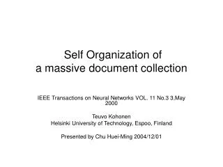
Self Organization of a Massive Document Collection Teuvo Kohonen Samuel Kaski Krista Lagus Jarkko Salojarvi Jukka Honkela Vesa Paatero Antti Saarela
Their Goal • Organize large document collections according to textual similarities • Search engine • Create a useful tool for searching and exploring large document collections
Their Solution • Self-organizing maps • Groups similar documents together • Interactive and easily interpreted • Facilitates data mining
Self-organizing maps • Unsupervised learning neural network • Maps multidimensional data onto a 2 dimensional grid • Geometric relations of image points indicate similarity
Self-organizing map algorithm • Neurons arranged in a 2 dimensional grid • Each neuron has a vector of weights • Example: R, G, B values
Self-organizing map algorithm (cont) • Initialize the weights • For each input, a “winner” is chosen from the set of neurons • The “winner” is the neuron most similar to the input • Euclidean distance: sqrt ((r1 – r2)2 + (g1 – g2)2 + (b1 – b2)2 + … )
Self-organizing map algorithm (cont) • Learning takes place after each input • ni(t + 1) = ni(t) + hc(x),i(t) * [x(t) – ni(t)] • ni(t) weight vector of neuron i at regression step t • x(t) input vector • c(x) index of “winning” neuron • hc(x),i neighborhood function / smoothing kernel • Gaussian • Mexican hat
Self-organizing map example 6 shades of red, green, and blue used as input 500 iterations
The Scope of This Work • Organizing massive document collections using a self-organizing map • Researching the up scalability of self-organizing maps
Original Implementation • WEBSOM (1996) • Classified ~5000 documents • Self-organizing map with “histogram vectors” • Weight vectors based on collection of words whose vocabulary and dimensionality were manually controlled
Problem • Large vector dimensionality required to classify massive document collections • Aiming to classify ~7,000,000 patent abstracts
Goals • Reduce dimensionality of histogram vectors • Research shortcut algorithms to improve computation time • Maintain classification accuracy
Histogram Vector • Each component of the vector corresponds to the frequency of occurrence of a particular word • Words associated with weights that reflect their power of discrimination between topics
Reducing Dimensionality • Find a suitable subset of words that accurately classifies the document collection • Randomly Projected Histograms
Randomly Projected Histograms • Take original d-dimensional data X and project to a k-dimensional ( k << d ) subspace through the origin • Use a random k x d matrix R, the elements in each column of which are normally distributed vectors having unit length: Rk x d Xd x N => new matrix Xk x N
Why Does This Work? • Johnson – Lindenstrauss lemma: “If points in a vector space are projected onto a randomly selected subspace of suitably high dimension, then the distances between the points are approximately preserved” • If the original distances or similarities are themselves suspect, there is little reason to preserve them completely
In Other Words • The similarity of a pair of projected vectors is the same on average as the similarity of the corresponding pair of original vectors • Similarity is determined by the dot product of the two vectors
Why Is This Important? • We can improve computation time by reducing the histogram vector’s dimensionality
Optimizing the Random Matrix • Simplify the projection matrix R in order to speed up computations • Store permanent address pointers from all the locations of the input vector to all locations of the projected matrix for which the matrix element of R is equal to one
So… • Using randomly projected histograms, we can reduce the dimensionality of the histogram vectors • Using pointer optimization, we can reduce the computing time for the above operation
Map Construction • Self-organizing map algorithm is capable of organizing a randomly initialized map • Convergence of the map can be sped up if initialized closer to the final state
Map Initialization • Estimate larger maps based on the asymptotic values of a much smaller map • Interpolate/extrapolate to determine rough values of larger map
Optimizing Map Convergence • Once the self-organized map is smoothly ordered, though not asymptotically stable, we can restrict the search for new winners to neurons in the vicinity of the old one. • This is significantly faster than performing an exhaustive winner search over the entire map • A full search for the winner can be performed intermittently to ensure matches are global bests
Final Process • Preprocess text • Construct histogram vector for input • Reduce dimensionality by random projection • Initialize small self-organizing map • Train the small map • Estimate larger map based on smaller one • Repeat last 2 steps until desired map size reached
Performance Evaluation • Reduced dimensionality • Pointer optimization • Non-random initialization of the map • Optimized map convergence • Multiprocessor parallelism
Largest Map So Far • 6,840,568 patent abstracts written in English • Self-organizing map composed of 1,002,240 neurons • 500-dimension histogram vectors (reduced from 43,222) • 5 ones in each column of the random matrix
Conclusions • Self-organizing maps can be optimized to map massive document collections without losing much in classification accuracy