Download
1 / 113
1.13k likes | 1.14k Views
This article discusses the estimation of the spectral density function for a weakly stationary time series using the autocovariance function. It also covers complex number results and expectations, variances, and covariances of linear and quadratic forms. The Discrete Fourier Transform is introduced for estimating the spectral density function.

E N D
The spectral density function, f(l) The spectral density function, f(x), is a symmetric function defined on the interval [-p,p] satisfying and The spectral density function, f(x), can be calculated from the autocovariance function and vice versa.
Expectations of Linear and Quadratic forms of a weakly stationary Time Series
Theorem Let {xt:tT} be a weakly stationary time series. Let Then and where and Sr = {1,2, ..., T-r}, if r ≥ 0, Sr = {1- r, 2 - r, ..., T} if r ≤ 0.
Also since Q.E.D.
Theorem Let {xt:tT} be a weakly stationary time series. Let and
Then where and Also Sr= {1,2, ..., T-r}, if r ≥ 0, Sr = {1- r, 2 - r, ..., T} if r ≤ 0.
Theorem Let {xt:t T} be a weakly stationary time series. Let Then
and Sr = {1,2, ..., T-r}, if r ≥ 0, Sr = {1- r, 2 - r, ..., T} if r ≤ 0, k(h,r,s) = the fourth order cumulant = E[(xt - m)(xt+h - m)(xt+r - m)(xt+s - m)] - [s(h)s(r-s)+s(r)s(h-s)+s(s)s(h-r)] Note k(h,r,s) = 0 if {xt:t T}is Normal.
Theorem Let {xt:t T} be a weakly stationary time series. Let Then
where and
Examples The sample mean
Thus and
and where
Thus Compare with
If g(•) is a continuous function then: Basic Property of the Fejer kernel: Thus
The sample autocovariancefunction The sample autocovariance function is defined by:
or if m is known where
or if m is known where
Theorem Assume m is known and the time series is normal, then: E(Cx(h))= s(h),
Proof Assume m is known and the the time series is normal, then: and
and Finally
Let x1,x2,x3, ...xT denote T observations on a univariate one-dimensional time series with zero mean (If the series has non-zero mean one uses in place of xt). Also assume that T = 2m +1 is odd. Then
where with lk = 2pk/T and k = 0, 1, 2, ... , m.
The Discrete Fourier transform: k = 0, 1,2, ... ,m.