Download

1 / 23
230 likes | 326 Views
Discover a faster, reliable algorithm to estimate p-values of Multinomial LLR Statistic in bioinformatics and other fields. Compare Hertz and Stormo’s method with Baglivo et al.’s approach. Enhance accuracy, overcome numerical errors, and optimize runtime by shifting values. Implement FFT-based convolution for efficiency. Achieve high scalability and exceptional accuracy in computational results.

E N D
A faster reliable algorithm to estimate the p-value of the multinomial llr statistic Uri Keich and Niranjan Nagarajan (Department of Computer Science, Cornell University, Ithaca, NY, USA)
Is there a motif here? • Is the alignment interesting/significant? • Which of the columns form a motif? Or for that matter here?
Uncovering significant columns • Work with column profiles • Null hypothesis: multinomial distribution where for a random sample of size Test Statistic: Log-likelihood ratio Calculate p-value of the observed score s
and more … • Bioinformatics applications: • Sequence-Profile and Profile-Profile alignment • Locating binding site correlations in DNA • Detecting compensatory mutations in proteins and RNA • Other applications: • Signal Processing • Natural Language Processing
Computational Extremes! • Asymptotic approximation • As, • Direct enumeration • Constant time approximation • Fails with N fixed and s approaching the tail • possible outcomes • Exact results • Exponential time and space requirements (O(NK)) even with pruning of the search space!
The middle path • Compute pQ the p.m.f. of the integer valued (Baglivo et al, 1992) where is the mesh size. • Runtime is polynomial in N, K and Q • Accurate upto the granularity of the lattice
Baglivo et al.’s approach • Compute pQ by first computing the DFT! Let and then, Then recover pQ by the inverse-DFT But how do we compute the DFT in the first place without knowing pQ??
Hertz and Stormo’s Algorithm • Sample from which are independent Poissons with mean (instead of X) Fact: We compute where Recursion:
Baglivo et al.’s Algorithm • Recurse over k to compute DFT of Qk,n • Let DQk,n be . Then, • And is upto a constant
Comparison of the two algorithms • Both have O(QKN2) time complexity • Space complexity: • O(QN) for Hertz and Stormo’s method • O(Q+N) for Baglivo et al.’s method • Numerical errors: • Bounded for Hertz and Stormo’s method. • Baglivo et al.’s method can yield negative p-values in some cases!
Whats going wrong? • Hoeffding (1965) proved that P(I s) f(N,K)e-s • If we compare with we would get …
And why? • Fixed precision arithmetic: • In double precision arithmetic • Due to roundoff errors the smaller numbers in the summation in the DFT are overwhelmed by the largest ones! • Solution: boost the smaller values • How? • And by how much?
Our Solution • We shift pQ(s) with es: where is the MGF of IQ • To compute the DFT of p we replace the Poisson pk with and compute
Which to use? • With = 1, N = 400, K = 5,
Optimizing • Theoretical error bound Want to calculate P(I > s0) and so a good choice for seems to be We can solve for numerically. This only adds O(KN2) to the runtime.
So far … • We have shown how to • compensate for the errors in Baglivo et al.’s algorithm • provide error guarantees • As a bonus we also avoid the need for log-computation! • The updated algorithm has O(Q+N) space complexity. • However the runtime is still O(QKN2) • Can we speed it up?
A faster variant! • Note that the recursive step is a convolution • Naïve convolution takes time O(N2) • An FFT based convolution, takes O(NlogN) time! • Unfortunately the FFT based convolution introduces more numerical errors: • When =1,
The final piece • Need a shift that works well on both and • The variation over l is expected to be small. So we focus on computing the correct shift for different values of k. • We make an intuitive choice where Mk(2) is the MGF of
Experimental Results (Accuracy) • Both the shifts work well in practice! • We tested our method with K values upto a 100, N upto 10,000 and various choices of and s • In all cases relative error in comparison to Hertz and Stormo was less than 1e-9
Experimental Results (Runtime) • As expected, our algorithm scales as NlogN as opposed to N2 for Hertz and Stormo’s method!
Recovering the entire range • Imaginary part of computed p is a measure of numerical error • Adhoc test for reliability: Real(p(j)) > 103× maxj Imag(p(j)) • In practise, we can recover the entire p.m.f. using as few as 2 to 3 different s (or equivalently ) values. • For large Ns this is still significantly faster than Hertz and Stormo’s algorithm.
Work in progress … • Rigorous error bounds for choice of 2’s • Applying the methodology to compute other statistics • Extending the method to automatically recover the entire range • Exploring applications