Download
1 / 59
590 likes | 602 Views
Polarimetric shapes of spectral lines in solar observations. Egidio Landi Degl’Innocenti Dipartimento di Fisica e Astronomia Università di Firenze, Italia. 9th Serbian Conference on Spectral Line Shapes in Astrophysics. Banja Koviljaca, May 13-17, 2013. Line shapes I.

E N D
Polarimetric shapes of spectral lines in solar observations Egidio Landi Degl’Innocenti Dipartimento di Fisica e Astronomia Università di Firenze, Italia 9th Serbian Conference on Spectral Line Shapes in Astrophysics Banja Koviljaca, May 13-17, 2013
Line shapes I Whether thereis no doubt of what is the meaning of a “line shape” in the classical world of traditional spectroscopic observations, on the contrary, when speaking about “polarimetric line shapes” it is necessary to start by clarifying what we really mean by these words, namely what is indeed a “polarimetric line shape”. There is here some ambiguity because a real result of a measurement is always a recording, on a series of pixels, of a signal which is proportional to the intensity of radiation. If no polarimetric device is introduced, when observing an astronomical object, like the sun or a star, one generally gets a familiar profile with the intensity forming a kind of dip, like the remarkable ones shown in the following slide.
Line shapes II The most prominent lines of the solar spectrum: calcium II (H and K), sodium (D1 and D2), and Hα. (From Beckers, solar atlas)
Line shapes III When performing polarimetric observations the situation changes. To find the polarization signal the observer is obliged to perform at least two observations and then to compare them in order to extract the polarization signal. This example is taken from Hale (1908). (Fe I line, g=1,83) Spectra (2) and (3) are relative to a sunspot observed in two directions of polarization
Line shapes IV George Ellery Hale was indeed the first, in 1908, to perform spectro-polarimetric observations of a celestial body, in partilcular of the sun. Thirteen years earlier (1895) Zeeman had discovered in the laboratory the effect which brings his name and Hale had the idea of employing it in solar observations, to see whether sunspots were indeed harboring magnetic fields, as it was suspected from Hα images of the chromosphere, showing what were called, at that time, the observed “vortices” surrounding sunspots. For his research Hale used a Nicol prism (acting as a polarizer) and a Fresnel rhomb (acting as a retarder). By changing the direction of the axis of the rhomb he was basically capable of measuring the circular polarization of radiation, thus discovering the presence of B on the sun.
Line shapes V Obviously, things have enormously evolved since the pioneering work of Hale, but even today, when measuring polarization, we are always obliged to refer to the difference of two separate, spectroscopic images obtained by changing some polarimetric device in the telescope optical train in such a way to alter the polarization characteristics of the observed radiation in a known way. A “spectropolarimetric profile” thus remains something that is vaguely defined, unless referring to a set of conventions and definitions. Fortunately, today we can make use of a convention that is almost universally accepted (at least for observations in the visible, UV and IR). This convention is based on the Stokes parameters.
Line shapes VI The Stokes parameters where introduced in the scientific literature as early as 1852. By means of their definition, which implies a statistical average of the electromagnetic signal associated with a radiation beam, it was possible to get a fully satisfactory description of polarization. In particular, through the operational definition given by Stokes, it was possible to correctly describe in mathematical terms even an unpolarized radiation beam. This was not at all trivial. In prior formulations, like e.g. the one used by Fresnel, which only considered pure monochromatic waves, the radiation always resulted in being 100% polarized... One has to wait, however, for more than a century before these quantities start being used in a systematic way in theoretical and observational astrophysics.
Line shapes VII With no doubt this is due to the seminal paper of Unno (1958) who was the first to establish a radiative transfer equation for the Stokes parameters in a stellar atmosphere. Since then, Stokes parameters have entered the jargon of astrophysics (in particular of solar physics) and it is now fairly well acknowledged that, when we speak about a spectropolarimetric profile, we have to speak about the profiles of the four Stokes parameters as a function of wavelength (or as a function of frequency). What is a single plot in traditional spectroscopy, I(λ), then becomes in general a set of four plots: I(λ), Q(λ), U(λ), and V(λ).
Line shapes VIII However, it has to be well kept in mind that Stokes parameters always rely on specific conventions, since they are defined with respect to a “reference direction” that has to be selected by the observer once and for all. Moreover, there are two further conventions that enter their definition and which specify the sign for the 3rd and the 4th parameter. This is schemtically summarized in the figure. Radiation is coming from behind the screen.
Line shapes IX It has to be remarked that the convention summarized in the previous figure seems to be more and more adopted today, with the exception of radioastronomers who prefer to give the opposite definition for circular polarization.... From now on, we will refer to the "polarimetric shapes" of spectral lines as the profiles of the Stokes parameters as a function of wavelength (or frequency). The first instrument capable of producing such profiles was the "legendary" Stokes I scanning polarimeter installed at the prime focus of the 40 cm coronograph at the Sacramento Peak Observatory (House, Baur & Hull, 1976, Solar Phys. 45, 495). Indeed, it was very slow (the polarimetric analysis was done a pixel at a time) but... it was the first...
Zeeman effect profiles I The first observations that came out from this instrument were very interesting but they were restricted to those targets that were presenting a fairly large amount of polarization, in particular sunspots. Only later, with the advent of better polarimetric techniques, other solar structures were targeted, like for instance prominences, where the polarization signal is much lower (≈ 1% instead of 10-20% typical of the umbrae of sunspots).
Zeeman effect profiles II Example of the polarimetric profiles obtained from Stokes I in two different points of a sunspot. Fe I line at 6173.5 Å (geff=2.5). Spectral resolution ≈ 1 arcsec
Zeeman effect profiles III The graphs shown in the previous slide are well representative of the polarimetric line profiles observed in a sunspot. Whereas a "traditional" line profile (the intensity profile) depends on the usual spectroscopic factors, namely 1. the strength of the line (proportional to the element, or ion abundance and to the oscillator strength); 2. the damping constant (due to natural broadening and to collisional broadening); 3. the run of the physical parameters (like temperature, pressure and r.m.s. velocity) in the line forming region; the polarimetric profiles also depend on the magnetic field vector (intensity and direction), and on other atomic properties, like the Zeeman pattern, of the spectral line.
Zeeman effect profiles IV The shape of polarimetric profiles changes with the magnetic field and this is just the property that has been used over the years for the diagnostics of magnetic fields in the sun and stars. Inded, the intensity of the magnetic field could be simply derived, at least in principle, by measuring the wavelength shifts of the different Zeeman components. Unfortunately, this procedure, widely used in the laboratory, can be applied only in very few special cases of astrophysical interest because the Zeeman splitting is generally on the same order of magnitude, if not lower, than the typical shifts introduced by the other mechanisms which contribute to the broadening of the lines (like Doppler shifts due to thermal or turbulent velocities, collisions, etc.).
Zeeman effect profiles V Polarimetric line shapes then result in being of fundamental importance for the diagnostics of the magnetic field. One can simply state that, without polarimetry, it is practically impossible to have even an estimate of B in astronomical objects. But, which are the typical signatures introduced by the magnetic field in polarimetric profiles through the Zeeman effect? There are indeed some general rules that can be stated. However, for practical applications, one has to rely on rather restrictive hypotheses about the nature itself of the magnetic field in the outermost layers of the sun (or of a star).
Zeeman effect profiles VI In a typical spectropolarimetric observation what is observed is a signal resulting from an average over a resolution element of the solar atmosphere, over the sampling time, and over a wavelength interval fixed by the resolution of the spectrometer. This signal obviously conveys some information about the magnetic field, but what is the magnetic field that we are speaking about? Is the magnetic field indeed constant over the resolution element and over the sampling time? If the polarimetric signal would vary linearly with B then we could hope to measure a kind of average. But the signal is highly non linear... Moreover, is the magnetic field a pure deterministic quantity, or does it present a kind of chaotic behavior, typical of a turbulent medium?
Zeeman effect profiles VII These are the typical questions that are now debated by the scientific community and,as stated earlier, we have to rely on assumptions to obtain physical results. The simplest, but highly questionable assumption is that the magnetic field is deterministic and that it is constant in time and over the resolution element. Even under these restrictive assumption, and even adding the further assumption of neglecting velocity fields, a real plethora of polarimetric profiles can result. This is obvious if we just think that such profiles, differently from the usual intensity profiles, depend on three extra-parameters (the three components of the magnetic field vector) that add to the "traditional" ones.
Zeeman effect profiles VIII In order to interpret such profiles and to proceed to a diagnostics of solar magnetic fields, a research field has been opened in solar physics, the so-called field of "solarmagnetometry". In the course of the years, several techniques have been developed by many people working on this subject with the aim of extracting from the observed Stokes profiles a "measurement" of the solar vector magnetic field. The oldest ones were the magnetographic techniques (either longitudinal or transversal). Further techniques were those based on the bisector and on the center of gravity of the circular polarization profiles, those based on the fit to the Stokes profiles of simplified analytical solutions of the transfer equation (Unno-fit techniques), the so-called SIR technique (Stokes Inversion based on Response functions), forward modelling techniques, etc,
Zeeman effect profiles IX Probably, the most reliable one among all these methods of inversion is the "longitudinal magnetograph" technique, in as far as the magnetic field is weak (Zeeman shift << Doppler broadening) and the longitudial component of the magnetic field can be assumed to be constant. In this limiting case one can prove a kind of "theorem" (one of the few fully analytical results of radiative transfer for polarized radiation) which states that the circular polarization profile (V-Stokes parameter) is proportional to the derivative of the intensity profile I'(λ). V(λ)= - λ2e02Bpar/(4π m c2) geff I'(λ) where Bpar is the longitudinal component of the (weak) magnetic field and geff is the effective Landé factor.
Zeeman effect profiles X However, in many cases the magnetic field is not at all weak, and the other techniques have to be invoked. Here is an example of an Unno-fit to the profile of a FeI line at λ6302.5 (ASP data) observed in a sunspot. B = 0.213 T, θ = 128° Χ = 22°
Zeeman effect profiles XI The example shown is very nice, but it is not at all typical. Even in the umbrae of sunspots, where the assumption of a costant, deterministic magnetic field seems most appropriate, it is often difficult to find a reasonable fit to the observations. For want of anything better, it has been introduced since many years the idea of a "filling factor", or a quantity, f, that represents the fraction of the observed area covered by a uniform magnetic field, the remaining fraction, (1 - f), being field-free (or non–magnetic). Obviously, the fit to the observations usually results in being better (... a parameter having been added to the fitting prcedure ...) but the situation cannot be considered as fully satisfactory.
Zeeman effect profiles XII The situation gets much worser when observing either the penumbrae of sunspots or, with the more performant polarimeters now available (Hinode SOT/SP), capable of attaining a very high polarimetric sensitivities at high spatial resolution of 0.3 arcsec, even the quiet solar photosphere. The penumbrae of sunspots are permeated by very high velocity fields (Evershed effect). These fields introduce relevant asymmetries in the polarimetric profiles and the diagnostics of the magnetic field results in being more complicated showing correlations between v and B. The Hinode data have revealed that even the quiter regions of the solar atmosphere harbor weak magnetic fields on which a strong debate is now going on.
Zeeman effect profiles XIII The Hinode data have revealed the presence of ubiquitos magnetic fields in the quiet solar atmosphere. The value of 〈 | B | 〉, the average of the absolute value of the magnetic field, is on the order of 10 Gauss in the internetwork regions. The field seems also to be fairly inclined with respect to the vertical in the same regions. This result follows from the fact that in more than 70% of the pixels, a clear signal of linear polarization (Q and U) is observed, in many cases comparable with the V signal. Since for weak fields the linear polarization signal scales as the square of the magnetic field intensity, while V scales linearly, it seems that the only way out to interpret the observations is to suppose that magnetic fields are fairly inclined.
Zeeman effect profiles XIV An alternative explanation is that the magnetic field in the sun shows, at least partially, a kind of turbulent behavior. But turbulence is an ugly beast According to an apocryphal story, Horace Lamb (the author of one of the most wonderful books on Hydrodynamics) is quoted saying, in a speech to the British Association for the Advancement of Science: "I am an old man now and when I die and go to heaven, there are two matters on which I hope for enlightment. One is Quantum Electrodynamics and the other is the turbulent motion of fluids. About the former I am rather optimistic..." Lamb was referring to hydrodynamc turbulence. MHD turbulence is even worse.....
Zeeman effect profiles XV Nothing better that this drawing of Leonardo da Vinci (circa 1510) can explain intuitively what is turbulence. Do we have to think that, on the sun, the magnetic field has a similar behavior?
Zeeman effect profiles XVI Hopefully, this is not the case, but there are some indirect indications that something peculiar is "happening" to the solar magnetic field. Many researchers have indeed tried to measure, through spectropolairmetric observations, the gradient of the longitudinal component of the magnetic field along the vertical axis. These measurements, combined with simpler measurements of the lateral gradient of the horizontal component of the magnetic field, point to the result that, in sunspots umbrae, div B ≠ 0. Do we have to think that in the solar atmosphere there are magnetic monopoles? More probably, some componets of B are hidden in the form of turbulent fields.
Scattering polarization I But the Zeeman effect is not the only mechanism that can produce polarization in solar spectral lines. There is are another physical phenomenon capable of doing so, scattering polarization. The physical laws controlling this phenomenon have been first derived by means of classical approaches, and then generalized to account for quantum mechanics. In the simplest case of a two level atom whose lower level is "naturally" populated, each spectral line can be characterized by a polarizability factor, usually denoted by the symbol W2, which depends on the atomic properties of the line.
z y x Scattering polarization II This phenomenon can be observed in the solar spectrum by observing either the outermost layers of the sun (like prominences and the corona) or observing directly the disk at close distances from the limb (limb polarization). The fundamental ingredient for limb polarization is the anisotropy of the photospheric radiation field (due to geometry or to limb-darkening). An important property of scattering polarization is that it can be modified by the presence of a magnetic field (Hanle effect). It results in a further diagnostic tool for B.
Reference direction The Second Solar Spectrum Second Solar Spectrum(Ivanov, 1991): linearly polarized spectrum of the solar radiation coming from quiet regions close to the limb. A. Gandorfer, “The Second Solar Spectrum”, Vol II, 2002. Observation close to the south solar pole, 5 arcsec inside the limb.
Resonance polarization III The correct observation of the second solar spectrum has been made possible by the development of technolgies in the construction of polarimetesrs. In the early days of polarimetry, let us say in the years 1970 or so, it was difficult to obtain spectro-polarimetric measurements capable of reaching a sensitivity on the order of 1/1000. Nowadays, when the signal is integrated over an area of the solar surface on the order of 100 pixels, modern polarimeters can reach the sensitivity of 1 part over 100,000. This precision is necessary for the investigation of the second solar spectrum. Note that for the second solar spectrum it has becom customary to express the polarimetric profiles by giving the ratio Q/I as a function of wavelength (obviously U=V=0).
Wiehr (1975) Stenflo, Baur, & Elmore (1980) Stenflo, & Keller (1997) Resonance polarization IV Observational improvements: from 1975 to 1997
Resonance polarization V In the following slides I will present some typical results on the polarimetric line shapes observed in the second solar spectrum. All the graphs shown are taken from the atlas of Gandorfer. In a simple-minded approach, one may expect that each line would produce a polarization profile proportional to the polarizability factor, W2, of the line itself. In the early days, when these observations were planned and then started, there was some optimism. One could think of being capable of extracting from observations some indications about the "turbulent" magnetic filed permeating the quiet solar atmosphere. But the real observations showed many aspects that are still far from being explained in a satisfactory way.
Observations Gandorfer atlas II (Violet + UV) 3900 – 4600 Å
Observations Gandorfer atlas I 4600 – 7000 Å
Detail n.1 region around CaII K (3933) and H (3968)
Ca II interferences From Stenflo, A&A 84,68 (1980) This typical feature of the second solar spectrum had been discovered in 1980 by J.O. Stenflo. It is interpreted as the result of "quantum interference" between two different processes: scattering of the photon in the H line and scattering of the photon in the K line. In some way it is the analogue of the well known double-slit Young experiment. There are further examples of these interference patterns in the second solar spectrum.
Detail n.2 region around Fe I multiplet n. 43 and Sr II 4078
Detail n.3 region around Ca I 4227 The "gold medal of polarization"
Detail n.3 bis region around Ca I 4227 with normal spectrum superimposed
Historical remark This was indeed the first spectral line for which limb polarization was detected by R.O. Redman in 1941 (Monthly Notices of the R.A.S. 101, 266) . The two, almost superimposed lines refer to observations of the spectrum obtained with a Nicol polarizer set parallel or perpendicular to the limb. Unfortunately the line is severely blended.
Detail n.4 region around Ba II 4554 and Sr I 4607
Detail n.4bis region around Sr I 4607 The "silver medal" of polarization
Detail n.5 region around Ti I lines 4743, 4758, 4759
Detail n.6 region around Ba I 5535, and Ti I 5565, 5644 also visible a molecularr band of C2
Detail n.7 region around Na I D1 and D2 lines
Detail n.8 region around Hα
General charactersitics The general features of the second solar spectrum are the following: 1. Of the more than 10,000 lines present in the "usual" spectrum, only few produce remarkable polarization signals. Interestingly, many of these lines are due to elements that can be considered as "minor species", such as Europium, Neodynium, Dysprosium, etc., or to molecules (C2, MgH, CN). 2. Many lines have a depolarizing behavior (they have polarization signals lower than the continuum) 3. Whereas in the intensity spectrum the shapes of the lines are similar, in the polarization spectrum the shapes are of different types, which allows a suitable classification.
A classification scheme (Belluzzi and Landi Degl'Innocenti, 2009) According to their shape, polarization signals can be classified as S, W, or M, as shown in the examples below.
Results: formulation of 3 empirical laws 1. Properties of the lower level Law #1: “The lower level of the most polarizing lines of the second solar spectrum is either the ground level, or a metastable level or, alternatively, an excited level, which is the upper level of a resonance line producing a strong polarization signal”.
3. Properties concerning the quantum numbers Law #3: “The lines showing the strongest polarization signals (Q/I > 0.17%) are due to transitions having either ΔJ = +1, or ΔJ = 0, ΔJ being defined as Ju – Jl.” Results: formulation of 3 empirical laws 2. Correlations between classification and equivalent width Law #2: “All the selected signals produced by spectral lines having a small equivalent width (i.e. lines having Wl/l < 20 F) are of type S”.