Download
1 / 47
470 likes | 609 Views
2D FT Imaging. MP/BME 574. Frequency Encoding. Spatial Frequency (k). Time (t). Proportionality. FT. FT. Proportionality. Temporal Frequency (f). Position (x, or y). 2D Fast GRE Imaging. TE. G x. Phase Encode. Dephasing/ Rewinder. Asymmetric Readout. G y. Dephasing/ Rewinder.

E N D
2D FT Imaging MP/BME 574
Frequency Encoding Spatial Frequency (k) Time (t) Proportionality FT FT Proportionality Temporal Frequency (f) Position (x, or y)
2D Fast GRE Imaging TE Gx Phase Encode Dephasing/ Rewinder Asymmetric Readout Gy Dephasing/ Rewinder Gz Shinnar- LaRoux RF RF TR = 6.6 msec
Summary • Frequency encoding • Bandwidth of precessing frequencies • Phase • Incremental phase in image space • Implies shift in k-space • Entirely separable • 1D column-wise FFT • 1D row-wise FFT
k y Finish n k x Start 2D FT
k z k y n k x 3D FT Tscan =Ny Nz TR NEX i.e. Time consuming!
Zero-padding/Sinc Interpolation • Recall that the sampling theorem • Restoration of a compactly supported (band-limited) function • Equivalent to convolution of the sampled points with a sinc function
kz ky Case II • k-space: Image Space: FT
kz ky Case III Methods: Sampling • k-space: Image Space: FT
Case II Nyquist Case III Corner
kz ky Case II: Zero-filled • k-space: Image Space: FT
kz ky Case III: Zero-Filled Methods: Sampling • k-space: Image Space: FT
Case II: Nyquist Zero-filled Case III: Corner Zero-filled
Apodization • Rect windowing implies covolution with a truncated sinc function leading to Gibbs’ Ringing • Desire to smooth the windowing function so as to diminish ringing. • Gaussian is one option discussed by Prof. Holden • MRI often uses “Fermi” Filter:
Point Spread Functions Un-windowed: Radial Window:
Ref Corners Radial
= 45º Experimental Results Methods: Point response function 0 Degrees 45 Degrees
Summary • Samples in 2D k-space represent 2D sinusoids at specific harmonics and at specific rotation angles • Interpolation by zero-filling leads to: • Reduced partial volume artifact • Increased spatial resolution at specific angles • Role of Apodization window • Increases SNR • Decreases ringing artifact • Choice effects the angular symmetry of the PSF
Point response function due to time-dependent contrast • Example showing mapping on contrast-enhanced signal to model the point response function • Predict attainable resolution • Application to carotid artery MR angiography
Point Spread Function (PSF) Analysis • Step 1: Measure enhancement curves in patients • Step 2: Map enhancement curves to k-space • Step 3: Transform result to image space to obtain the point spread function
Fitted Two Phase Gamma Variate 160 140 Composite Fit First Pass Fit 120 Residual Fit 100 Measured Data Contrast Enhancement 80 60 40 20 0 0 10 20 30 40 50 60 70 80 Time (sec) Step 1: Enhancement Model
k z High Detail Information Start k y Overall Image Contrast Sampled Points Finish Step 2: Mapping to k-Space
Step 2: Mapping to k-Space k-Space Weighting -1 0.06 Measured Data 0.05 Composite k-Space First Pass Only Residual 0.04 Contrast Enhancement (sec) 0.03 0.02 0.01 0 0 0.05 0.1 0.15 0.2 0.25 0.3 0.35 0.4 0.45 0.5 Spatial Frequency (cycles/mm)
Analytical PSF for Fitted Curve 0.05 Spatial Resolution Composite PSF 0.04 First Pass PSF 0.03 Residual PSF Image Contrast PSF Amplitude (mm-sec 2 )-1 0.02 0.01 0 -0.01 0 0.5 1 1.5 2 2.5 3 3.5 4 4.5 5 Radius (mm) Step 3: Transform to Image Space
Analysis: Spatial Resolution × × FOV FOV TR y z FWHM 2 t1 p × Full Width at Half Maximum (FWHM) of the Point Spread Function is given by: • where, • FOVyand FOVzare the phase encoding Fields of View • TR is the repetition time • t1 is the time to peak enhancement of the bolus curve
Dependence of PSF on Acquisition Time 0.045 Infinite Scan 230 sec, Maximum Spatial Resolution 0.04 = 230 sec T acq T = 90 sec acq 1 0.035 T = 50 sec - acq T = 10 sec acq -sec) 0.03 2 90 0.025 Tacq = Acquisition Time in seconds 0.02 50 PSF amplitude (mm 0.015 10 0.01 0.005 0 0 0.5 1 1.5 2 2.5 3 3.5 4 Radius (mm) PSF Dependence on Acquisition Time
50 sec PSF Dependence on Acquisition Time Line Pairs/mm Acquisition Time (sec) 1.2 213 sec 90 sec 1.6 4.2 2.0 2.6 3.2 5.2 10 sec Z Y
Experiment: FOVz Reduction Z Y 13 cm X 6.4 cm 13 cm X 4.0 cm
Carotid and Vertebral Arteries: Acquisition Parameters • FOV: 22 cm (S/I) X 15 cm (R/L) X 6 cm (A/P) • Matrix: 256 X 168 X 40-44 • Acquired Voxel: 0.9 mm X 0.9 mm X 1.4 mm • 2X Zerofilling in all three directions • TR/TE 6.6 msec/1.4 msec • Acquisition Time: 44-51 seconds • 20 cc Gd
Acquisition Time: 11 sec 22 sec 33 sec 44 sec X X Z Z Left Carotid Artery Stenosis: Reconstruction at Multiple Time Points Coronal MIP, Full Data Set: MIP Reprojec-tions
Acquisition Time: 11 sec 22 sec 33 sec 44 sec X X Z Z Right Carotid Artery Stenosis: Reconstruction at Multiple Time Points
Partial k-Space Acquisition • Means of accelerating image acquisition at the expense of minor artifacts • ¾ k-space • ½ k-space -> Hermetian symmetry • Phase in the image space complicates matters • In practice, MR images have non-zero phase due to magnetic field variations • Susceptibility • General field inhomogeneity • “Homodyne” reconstruction required • Low spatial frequency estimation of the phase
FI = fftshift(fft(fftshift(I))); for i = 1:192, FI_34(i,:) =FI(i,:); end I_34 = fftshift(ifft(fftshift(FI_34))); figure;subplot(2,2,1),imagesc(abs(I_34));axis('image'); colorbar;colormap('gray');title('Magnitude') subplot(2,2,2),imagesc(angle(I_34));axis('image'); colorbar;colormap('gray');title('Phase') subplot(2,2,3),imagesc(abs(I-I_34));axis('image'); colorbar;colormap('gray');title('Error') gtext('Three-quarter k-space')
for i = 1:129, FI_Herm(i,:) =FI(i,:); end I_Herm = fftshift(ifft(fftshift(FI_Herm))); figure;subplot(2,2,1),imagesc(abs(I_Herm2));axis('image'); colorbar;colormap('gray');title('Magnitude') figure;subplot(2,2,1),imagesc(abs(I_Herm));axis('image'); colorbar;colormap('gray');title('Magnitude') subplot(2,2,2),imagesc(angle(I_Herm));axis('image'); colorbar;colormap('gray');title('Phase') subplot(2,2,3),imagesc(abs(I-I_Herm));axis('image');colorbar; colormap('gray');title('Error') gtext('One-half k-space')
count2 = 128; for i = 130:256, FI_Herm(i,:) =conj(FI(count2,:)); count2 = count2-1; end I_Herm2 = fftshift(ifft(fftshift(FI_Herm))); figure;subplot(2,2,1),imagesc(abs(I_Herm2));axis('image'); colorbar;colormap('gray');title('Magnitude') save phase_phantom subplot(2,2,2),imagesc(angle(I_Herm2));axis('image'); colorbar;colormap('gray');title('Phase') subplot(2,2,3),imagesc(abs(I-I_Herm2));axis('image'); colorbar;colormap('gray');title('Error') gtext('Hermetian k-space')
FIp = fftshift(fft(fftshift(IIII))); FIp_Herm = zeros(256); for i = 1:129, FIp_Herm(i,:) =FIp(i,:); end count2 = 128; for i = 130:256, FIp_Herm(i,:) =conj(FIp(count2,:)); count2 = count2-1; end Ip_Herm = fftshift(ifft(fftshift(FIp_Herm))); figure;subplot(2,2,1),imagesc(abs(Ip_Herm));axis('image'); colorbar;colormap('gray');title('Magnitude') subplot(2,2,2),imagesc(angle(Ip_Herm));axis('image'); colorbar;colormap('gray');title('Phase') subplot(2,2,3),imagesc(abs(I-Ip_Herm));axis('image'); colorbar;colormap('gray');title('Error') gtext('Attempt at Hermetian k-space for Image with Phase')