Download

1 / 75
760 likes | 911 Views
2D FT Review. MP/BME 574. 1D to 2D Sampling. Signal under analysis is periodic Signal is ‘essentially bandlimited’ Sampling rate is high enough to satisfy Nyquist criterion Other assumptions (for convenience) Signal is sampled with uniformly spaced intervals. n 2. n. 1.

E N D
2D FT Review MP/BME 574
1D to 2D Sampling • Signal under analysis is periodic • Signal is ‘essentially bandlimited’ • Sampling rate is high enough to satisfy Nyquist criterion • Other assumptions (for convenience) • Signal is sampled with uniformly spaced intervals
n2 n 1 2D Sampling/Discrete-Space Signal
2D Functions • Impulses • Step Sequences • Separable Sequences • Periodic Sequences
n2 n 1 Line Impulse
n 1 2D step n2
n2 n 1 2D step
n 1 2D Step n2
n 1 Separable Sequences n2
n2 n 1 Periodic Sequences
k2 (3) (4) (1) (2) k1 2D Convolution h(k1,k2) x(k1,k2) k2 k1
x(k1,k2) k2 k1 (2) (1) (4) (3) 2D Convolution h(-k1,-k2) k2 k1
x(k1,k2) k2 k1 (2) (1) (4) (3) 2D Convolution h(4-k1,3-k2) k2 3-k2 k1 4-k1
x(k1,k2) k2 k1 (2) (1) (4) (3) 2D Convolution h(n1-k1,n2-k2) k2 (2) (1) (4) (3) n2 k1 n1-1
(2) (1) (4) (3) 2D Convolution h(n1-k1,n2-k2) y(n1,n2) k2 n2 (7) (7) (4) (3) (4) n2 (6) (6) (4) n1 (2) k1 (1) (3) (3) n1-1
(2) (1) (4) (3) 2D Convolution h(n1-k1,n2-k2) y(n1,n2) k2 n2 (7) (7) (4) (3) (4) n2 (6) (10) (6) (4) n1 (2) k1 (1) (3) (3) n1-1
2DFT Imaging in MRI MP/BME 574
Abbe’s Theory of Image Formation From Meyer-Arendt
No Magnetic Field = No Net Magnetization Random Orientation
Dipole Moments from Entire Sample Magnetic Field (B0) Magnetic Field (B0) m m Positive Orientation Negative Orientation
Precession and Electromotive Force (emf) or Voltage • emf derives from Faraday’s law • Time-dependent magnetic flux through a coil of wire • Induces current flow • Proportional to the magnetic field strength and the frequency of the field oscillation
z B1(t) y x Example
z B1(t) y x Example
rf-excitation By reciprocity, Lab Frame Rotating Frame After Haacke, 1999
X X Quadrature Conversion in MRI (and Ultrasound) Signal Processing Received Radio Frequency Echo Signal x(t) (fc = 10MHz; 40MS/s) LPF xc(t) I—Channel 2 cos wct -p/2 Phase Shift -2 sin wct Q—Channel xs(t) LPF In a high-end ultrasound/MR imaging system this conversion is done in the digital domain. In a lower-end system the conversion is done in the analog domain. Why?
Slice Selection Ideal, non-selective rf: S(t) =rect(t/Dt) B1ideal(t)
Non-selective rf-pulse Entire Volume Excited
r Spatial Encoding Gradients z B(r) y x
Slice Selection Selective rf: Ssel(t) = sinc(t/t) rect(t/Dt) B1ideal(t) Apply spatial gradient simultaneous to rf-pulse.
Slice Selective rf-pulse Slice of width Dz Excited
Summary • Spin ½ nuclei will precess in a magnetic field Bo • Excite and receive signal with coils (antennae) by Faraday’s Law • Complex representation of real signals • Quadrature detection • Reciprocity • Spatial magnetic field gradients • Bandwidth of precessing “spins” • Non-Selective rf pulses using Fourier transform principles • Shift theorem etc… applies
r Spatial Encoding Gradients z B(r) y x
f, B Df B=Bo FOVx xmax xmin Frequency Encoding
Frequency Encoding Recall Lab 2, Problem 4: Piano Keyboard … … E, 660 Hz Middle C A, 220 Hz
Frequency Encoding Time (t) FT Proportionality Temporal Frequency (f) Position (x)
Spatial Frequency (k) Time (t) Proportionality FT FT Proportionality Temporal Frequency (f) Position (x) Frequency Encoding
f, B Df B=Bo FOVx xmax xmin Phase Encoding y
f, B Df B=Bo FOVx xmax xmin Phase Encoding y
f, B Df B=Bo FOVx xmax xmin Phase Encoding y
¶ B ¶ y Phase Encoding Zero gradient for time, T y
¶ B ¶ y Phase Encoding Positive gradient for time, T y
¶ B ¶ y Phase Encoding Positive gradient for time, T y
Frequency Encoding Spatial Frequency (k-ko) Time (t) Proportionality FT FT Proportionality Temporal Frequency (f) Position (x) e-igGyT