Download
1 / 8
80 likes | 201 Views
e. e. 3. 4. b. 3. b. 4. X. X. a. 1. 13. 4. a. 34. s. X. 45. |3. a. 3. 35. a. 23. X. X. 2. 5. b. e. 5. 5. OPTIONAL STEP: center each variable about its mean (X i -X i ). Path analysis and maximum likelihood estimation.

E N D
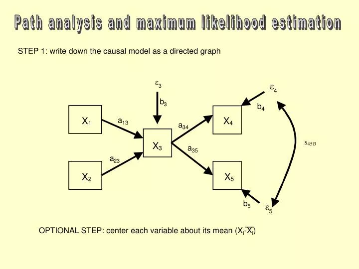
e e 3 4 b 3 b 4 X X a 1 13 4 a 34 s X 45 |3 a 3 35 a 23 X X 2 5 b e 5 5 OPTIONAL STEP: center each variable about its mean (Xi-Xi) Path analysis and maximum likelihood estimation STEP 1: write down the causal model as a directed graph
e e 3 4 b 3 b 4 X X a 1 13 4 a 34 s X 45 |3 a 3 35 a 23 X X 2 5 b e 5 5 Path analysis and maximum likelihood estimation Exogenous variables: variables that have no explicit causes in the model Endogenous variables: variables that are caused by other variables in the model
free parameter e e 3 4 b 3 b 4 X X a 1 13 4 a 34 s X 45 |3 a 3 35 a 23 X X 2 5 b e 5 5 Path analysis and maximum likelihood estimation STEP 2: translate this to a series of structured equations with free parameters X1=N(0,) 3=N(0,1) 5=N(0,1) X2=N(0,) 4=N(0,1) X3=a13X1+a23X2+b33 X4=a34X3+b44 X5=a35X3+b55 Cov(X1,X2)=Cov(X1,3)=Cov(X1, 4)=Cov(X1, 5)= Cov(X2,3)=Cov(X2, 4)=Cov(X2, 5)= Cov(3,4)=Cov(3, 5)=0 Cov(4, 5)=45
X1 X2 X3 X4 X5 X1 S1 0 a13S1 a13a34S1 a23a35S1 X2 S2 a23S2 a13a34S2 a23a35S2 X3 S3 a34S3 a35S3 X4 S4 a23S3+ b4b5Cov(4,5) X5 S5 = Path analysis and maximum likelihood estimation STEP 3: Derive the predicted variance and covariance between each pair of variables in the model, respecting the constraints implied by the causal graph, using covariance algebra.
Observed variances & covariances (S) Predicted variances & covariances ((free)) Path analysis and maximum likelihood estimation STEP 4: Estimate the free parameters by minimizing the difference between the observed and predicted variances and covariances. Maximum likelihood estimation Estimates of the free parameters (path coefficients,error variances, free covariances) that make the predicted covariance matrix() as close as possible to the observed variances and covariances, while respecting the constraints required by d-separation (I.e. the causal structure).
Path analysis and maximum likelihood estimation STEP 6: Look at the remaining differences between the observed and predicted covariance matrices, and calculate the probability of having observed this difference, assuming that these differences should be the same except for random sampling variation. X2ML (maximum likelihood chi-square statistic) degrees of freedom = V(V+1)/2 - #free parameters STEP 7: If the calculated probability is less than the chosen significance level (eg 0.05) then the data did not come from this causal process, and the model must be rejected; otherwise the data support the model.
Path analysis and maximum likelihood estimation Now, let's do some analyses... Using the EQS program
A B D C Path analysis and maximum likelihood estimation Overall association between X and Y Effects of causal ancestors on causal descendents Effects due to a common causal ancestor Unresolved causal relationships Direct effects Indirect effects