Download
1 / 45
750 likes | 3.24k Views
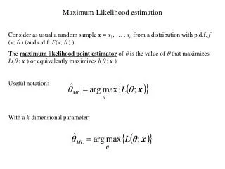
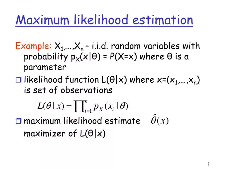
Maximum likelihood estimation. Example: X 1 ,…,X n – i.i.d. random variables with probability p X (x|θ) = P(X=x) where θ is a parameter likelihood function L(θ|x) where x=(x 1 ,…,x n ) is set of observations maximum likelihood estimate maximizer of L(θ|x).

E N D
Maximum likelihood estimation Example: X1,…,Xn – i.i.d. random variables with probability pX(x|θ) = P(X=x) where θ is a parameter • likelihood function L(θ|x) where x=(x1,…,xn) is set of observations • maximum likelihood estimate maximizer of L(θ|x)
typically easier to work with log-likelihood function, C(θ|x) = log L(θ|x)
Properties of estimators • estimator is unbiased if • is asymptotically unbiased if as n→∞
Properties of MLE • asymptotically unbiased, i.e., • asymptotically optimal, i.e., has minimum variance as n→∞ • invariance principle, i.e., if is MLE for θ then is MLE for any function τ(θ)
Network Tomography Goal: obtain detailed picture of a network/internet from end-to-end views • infer topology /connectivity
Network Tomography Goal: obtain detailed picture of a network/internet from end-to-end views • infer link-level • loss • delay • available bandwidth . . .
counting & projection brain model statistical model Maximum likelihood estimate perform inference inverse function problem data Brain Tomography unknown object
routing & counting queuing behavior binomial perform inference inverse function problem data Network Tomography
Why end-to-end • no participation by network needed • measurement probes regular packets • no administrative access needed • inference across multiple domains • no cooperation required • monitor service level agreements • reconfigurable applications • video, audio, reliable multicast
Di - one way delay D0 D2 D1 Naive Approach: I D0 +D1= M1 D0 +D2= M2 2 equations, 3 unknowns M2 M1 {Di} not identifiable
D’0 D0 D’2 D’1 D2 D1 D0 + D1 D0 +D2 Naive Approach: II • bidirectional tree
D0 D’0 D’2 D’1 D2 D1 D0 + D1 D0 +D2 Naive Approach: II • bidirectional tree D’2+ D1
D0 D’0 D’2 D’1 D2 D1 D0 + D1 D0 +D2 Naive Approach: II • bidirectional tree D’1+D2 D’2+ D1
D0 D2 D1 D0 + D1 D0 +D2 Naive Approach: II • bidirectional tree D’0 +D’1 D’0 +D’2 D’0 D’2 D’1 D’1+D2 D’2+ D1
D’0 +D’1 D’0 +D’2 D’0 D0 D’2 D’1 D2 D1 D0 + D1 D0 +D2 D’1+D2 D’2+ D1 Naive Approach: II • bidirectional tree • 6 equations, 6 unknowns • not linearly independent! (not identifiable)
A R0 R2 R1 B C Naive Approach: III Round trip link delays: RAB = R0 + R1 RAC = R0 + R2 RBC = R1+ R2 Linear independence! (identifiable) • true for general trees • can infer some link delays within general graph
Bottom Line • similar approach for losses • yields round trip and one way metrics for subset of links • approximations for other links
a1 a2 a3 MINC (Multicast Inference of Network Characteristics) • multicast probes • copies made as needed within network source • receivers observe correlated performance • exploit correlation to get link behavior • loss rates • delays receivers
α1 α2 α3 MINC (Multicast Inference of Network Characteristics) • multicast probes • copies made as needed within network • receivers observe correlated performance • exploit correlation to get link behavior • loss rates • delays
α1 x α2 α3 MINC (Multicast Inference of Network Characteristics) • multicast probes • copies made as needed within network • receivers observe correlated performance • exploit correlation to get link behavior • loss rates • delays
α1 x α2 α3 MINC (Multicast Inference of Network Characteristics) • multicast probes • copies made as needed within network • receivers observe correlated performance • exploit correlation to get link behavior • loss rates • delays
α1 α2 α3 MINC (Multicast Inference of Network Characteristics) • multicast probes • copies made as needed within network • receivers observe correlated performance • exploit correlation to get link behavior • loss rates • delays estimates of α1, α2, α3
Probe source • ak k Multicast-based Loss Estimator • tree model • known logical mcast topology • tree T = (V,L) = (nodes, links) • source multicasts probes from root node • set R V of receiver nodes at leaves • loss model • probe traverses link k with probability ak • loss independent between links, probes • data • multicast n probes from source • data Y={Y(j,i), j R, i=1,2,…,n} • Y(j,i) = 1 if probe i reaches receiver j, 0 otherwise • goal • estimate set of link probabilities a = {ak : k V} from data Y
Loss Estimation on Simple Binary Tree Source • each probe has one of 4 potential outcomes at leaves • (Y(2),Y(3)) { (1,1), (1,0), (0,1), (0,0) } • calculate outcomes’ theoretical probabilities • in terms of link probabilities {a1, a2, a3} • measure outcome frequencies • equate • solve for {a1, a2, a3}, yielding estimates • key steps • identification of set of externally measurable outcomes • knowing probabilities of outcomes knowing internal link probabilities 0 a1 1 a2 a3 2 3 Receivers
Probe source k receivers R(k) descended from k General Loss Estimator & Properties • Can be done, details see R. Cáceres, N.G. Duffield, J. Horowitz, D. Towsley, ``Multicast-Based Inference of Network-Internal Loss Characteristics,'' IEEE Transactions on Information Theory, 1999
Statistical Properties of Loss Estimator • model is identifiable • distinct parameters {ak } distinct distributions of losses seen at leaves • Maximum Likelihood Estimator • strongly consistent (converges to true value) • asymptotically normal • (MLE efficient [ minimum asymptotic variance])
Impact of Model Violation • mechanisms for dependence between packets losses in real networks • e.g. synchronization between flows from TCP dynamics • expect to manifest in background TCP packets more than probe packets • temporal dependence • ergodicity of loss process implies estimator consistency • convergence of estimates slower with dependent losses • spatial dependence • introduces bias in continuous manner: small correlation result in small bias • can correct for with a priori knowledge of typical correlation • second order effect • depends on gradient of correlation rather than absolute value
MINC: Simulation Results • accurate for wide range of loss rates • insensitive to • packet discard rule • interprobe distribution beyond mean inferred loss probe loss
MINC: Experimental Results • background traffic loss and inferred losses fairly close • over range of loss rates, best when over 1% inferred loss background loss
Validating MINC on a real network • end hosts on the MBone • chose one as source, rest as receivers • sent sequenced packets from source to receivers • two types of simultaneous measurement • end-to-end loss measurements at each receiver • internal loss measurements at multicast routers • ran inference algorithm on end-to-end loss traces • compared inferred to measured loss rates • inference closely matched direct measurement
experiments with 2- 8 receivers 40 byte probes 100 msec apart topology determined using mtrace kentucky atlanta cambridge SF edgar erlang LA saona WO conviction excalibur alps rhea MINC: Mbone Results
Topology Inference Probe source • problem • given • multicast probe source • receiver traces (loss, delay, …) • identify (logical) topology • motivation • topology may not be supplied in advance • grouping receivers for multicast flow control ? Receivers
General Approach to Topology Inference • given model class • tree with independent loss or delay • find classification function of nodes k which is • increasing along path from root • can be estimated from measurements at R(k) = leaves descended from k • examples • 1-Ak = Prob[probe lost on path from root 0 to k] • mean of delay Yk from root to node k • variance of delay Yk from root to node k • build tree by recursively grouping nodes {r1,r2,…,rm} • to maximize classification function on putative parent
BLTP Algorithm 1. construct binary tree based on losses • estimate shared loss L = 1-Akseen from receiver pairs • aggregate pair with largest L • repeat till one node left
Example 1. construct binary tree • estimate shared loss L seen from receiver pairs • aggregate pair with largest L • repeat till one node left
Example 1. construct binary tree • estimate shared loss L seen from receiver pairs • aggregate pair with largest L • repeat till one node left
Example 1. construct binary tree • estimate shared loss L seen from receiver pairs • aggregate pair with largest L • repeat till one node left
Example 1. construct binary tree • estimate shared loss L seen from receiver pairs • aggregate pair with largest L • repeat till one node left
Example 1. construct binary tree • estimate shared loss L seen from receiver pairs • aggregate pair with largest L • repeat till one node left
Example 1. construct binary tree • estimate shared loss L seen from receiver pairs • aggregate pair with largest L • repeat till one node left
Example 1. construct binary tree • estimate shared loss L seen from receiver pairs • aggregate pair with largest L • repeat till one node left
BLTP Algorithm 1. construct binary tree 2. prune links with 1-ak<e
Theoretical Result 1. construct binary tree 2. prune links with 1-ak<e if e < min 1-ak, topology identified with prob 1 as n
Results Simulation of Internet-like topology (min ak ~.12) BLTP is • simple, efficient • nearly as accurate as Bayesian methods • can combine with delay measurements
Issues and Challenges • relationship between logical and physical topology • relation to unicast • tree layout/composition • combining with network-aided measurements • scalability