Download
1 / 1
10 likes | 152 Views
M2.6. Testing Automated Solar Flare and Coronal Mass Ejection Forecasting With 13 Years of MDI Synoptic Magnetograms James P. Mason 1,2 , J. T. Hoeksema 2 1 University of California, Santa Cruz; 2 Stanford University. Poster 16.10. Abstract.

E N D
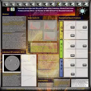
M2.6 Testing Automated Solar Flare and Coronal Mass Ejection Forecasting With 13 Years of MDI Synoptic MagnetogramsJames P. Mason1,2, J. T. Hoeksema21University of California, Santa Cruz; 2Stanford University Poster 16.10 Abstract This investigation uses the entire set of synoptic line-of-site magnetograms from the SOHO Michelson Doppler Imager (MDI) to calculate multiple characteristics of the magnetic field in active regions. These measures are calculated for the disk passage of 1075 NOAA active regions spanning Solar Cycle 23 from 1996 - 2009 in an attempt to determine the ability of line-of-sight magnetograms to be used as a predictor of coronal mass ejections (CMEs) and/or solar flares. Previous studies of this nature have been restricted to a relatively small sample size. This expansive study is accomplished by using an IDL code that automatically searches the MDI database for data related to any NOAA AR, identifies the primary neutral line on remapped data [Bokenkamp, 2007], applies a constant-alpha force-free field model [Allisandrakis, 1981], and calculates several measures of nonpotentiality [Falconer, 2008]. Superposed epoch plots were produced for these measures surrounding various “Key times” (see Analysis). These plots were used to seek out any pre- or post- flare signatures with the advantage of the capability to resolve weak signals. Superposed Epoch Analysis Solar Cycle 23 GWIL % Change -20 hr: 10.0% -40 hr: 22.2% % Change -20 hr: 15.8% -40 hr: 46.7% Our large sample size affords us the opportunity to get a sense for an entire solar cycle. Blue series roughly represent solar minimum, red: solar maximum, and green: declining phase. As expected, the max phase produces a lot more ARs with any and every value. % Change -20 hr: 11.1% -40 hr: 17.6% Eff. Sep. Key Lists Each Key List consists of a large number of user-specified Key Times. These Key Times become the t=0 point for each data series so that the data can be sensibly combined for multiple active regions. X: All X class flares. 98 total M: All M class flares. 1,139 total Quiet: ARs w/ only B-C class flares. 4,932 total Dead Silent: ARs with no flaring at all. 410 total Note: Keylists for flares can have >1 flare (Key time) per AR. % Change -20 hr: -13.6% -40 hr: -17.4% % Change -20 hr: -8.3% -40 hr: -9.9% Individual AR example: 8910 GWIL (Gradient Weighted Inversion Line Length): Shows a general “hill” trend around flares that is more pronounced for stronger flares. Largest % change for all parameters. Dead Silent (null) test shows decay consistent with aging ARs. Eff. Sep. (Effective Separation/Distance): Separation between flux weighted centers of ~bipolar active region. Displays an overall decrease in response to flare which is again, stronger for more powerful flares. Null test shows a constant values during disk passage implying little AR evolution in these relatively inactive active regions. Tot. Flux (Total Unsigned Flux): Exhibitsincrease in response to flare which is only moderately sensitive to flare strength. Implies energy storage. The null test shows that this may not be unique to flaring regions. Note: % changes are calculated from t=0 to indicated time. % Change -20 hr: -9.1% -40 hr: -10.7% Tot. Flux % Change -20 hr: 5.7% -40 hr: 17.4% % Change -20 hr: 5.3% -40 hr: 11.2% The only selection criterion imposed in this study is that the AR must be within 30 degrees of disk center to minimize projection errors. See right for description of parameters. The temporal location of an M2.6 flare is marked by a vertical bar (physical location indicated by point of lightning bolt at top of poster). The plots to the right show that the parameters have a strong response to the flare. But is this a typical response? Superposed Epoch (SPE) analysis can help answer this question. % Change -20 hr: 2.1% -40 hr: 2.0% References: Alissandrakis, C.E., 1981, Astron. Astrophys. 100, 197. Bokenkamp, N., 2007, Undergraduate Thesis. Bokenkamp, N., 2007, AAS Meeting 210, #93.24. Falconer, D.A. et al., 2003, Geophys. Res., 108,1380. Falconer, D.A. et al., 2008, ApJ, 689, 1433. Leka, K.D. & Barnes, G., 2003, ApJ, 595, 1277. Leka, K.D. & Barnes, G., 2006, ApJ, 656, 1173. . Conclusions forecasting. Further study will include the time variation of total flux (df/dt). Vector magnetograms provide the opportunity to calculate many more (perhaps more flare indicative) parameters. SDO will will be an excellent source for such data. While a flare response is evident in the above SPE plots, they lack the type of strong signal response required for accurate space weather The data output for every magnetogram included in this study were placed in a single table and made available to the public: http://soi.stanford.edu/~jmason86/GreatTable. There are 71,324 magnetograms included in our “Great Table”, each with their corresponding NOAA AR #, date, time, MDI fits file identifier, Carrington location, pixel size of sub-image, and 5 calculated variables.


