Download
1 / 23
230 likes | 412 Views
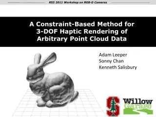
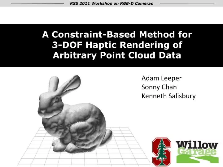
RSS 2011 Workshop on RGB-D Cameras. A Constraint-Based Method for 3-DOF Haptic Rendering of Arbitrary Point Cloud Data. Adam Leeper Sonny Chan Kenneth Salisbury. 1. Overview. Motivation Part One: Haptic Algorithm Part Two: Real-Time Strategies Results. Motivation.

E N D
RSS 2011 Workshop on RGB-D Cameras A Constraint-Based Method for 3-DOF Haptic Rendering of Arbitrary Point Cloud Data Adam LeeperSonny ChanKenneth Salisbury 1
Overview • Motivation • Part One: Haptic Algorithm • Part Two: Real-Time Strategies • Results
Motivation • Force feedback for teleoperation is costly to measure. • We can use a model to estimate interaction forces. • Remote sensors produce 3D points. 3
Potential Fields and Penalty Methods • Haptic force is computed from current HIP position. • Force is proportional to penetration depth. Geometric Shapes Infinite Wall F = -k*x x
Potential Fields and Penalty Methods • Haptic force is computed from current HIP position. • Force is proportional to penetration depth. “pop-through” when objects are thin
Constraint-Based Methods • A proxy / god-object is constrained to the surface. • A virtual spring connects proxy to HIP.
Some Previous Methods • Cha, Eid, Saddik. EuroHaptics 2008. • Depth-image tessellation. • Proxy mesh algorithm. • El-Far, Georganas, El Saddick. 2008. • Per-point AABB collision detection. • Proxy constrained to discrete point locations.
Constraint-Based Methods • Constraint method works well for implicit functions • Salisbury & Tarr, 1997 f < 0 f > 0 http://xrt.wikidot.com/
Constraint-Based Methods • A constraint-plane is given by the surface pointand normal.
From Points to an Implicit Surface • Great. So how do we make an implicit surface from points? • First, we’ll give each point a compact weighting function. • Then we have two options: • Metaballs: constructive geometry • Surfels: surface estimation
From Points to an Implicit Surface • Metaballs • Each point produces a 3D scalar field f(x,y,z). • The net scalar field is simply the sum of all points. • A threshold value, T, is chosen to define an isosurface on this field. T = 0.6 T = 0.2
From Points to an Implicit Surface • Metaballs • Each point produces a 3D scalar field f (x,y,z). • The net scalar field is simply the sum of all points. • A threshold value, T, is chosen to define an isosurface on this field. Don’t need point normals! T = 0.2 T = 0.6
From Points to an Implicit Surface • Metaballs • Each point produces a 3D scalar field f (x,y,z). • The net scalar field is simply the sum of all points. • A threshold value, T, is chosen to define an isosurface on this field.
From Points to an Implicit Surface • Surfels • Local surface estimation (Adamson and Alexa 2003) weighted-average point position weighted-average point normal
Selecting Parameters • Auto-generated parameters adapt easily to any input cloud! • For each point: • Compute the average distance, d, to the nearest N=3 neighbors. • Set R to some multiple m of d. Generally m ~= 2. • For metaball rendering, T = 0.5 – 0.8 works for most data.
Part Two: Real-Time Strategies • Fast Collision Detection • Spatial Issues • Temporal Issues
Fast Collision Detection • Haptic servo loop is typically 1kHz, can’t use all points! • Points have only compact support of radius R. • A kd-tree or octree provides fast radius and kNN searches.
Spatial Issues • 640x480 depth image = 300,000 points. • Some are outside the workspace of the haptic device. • Sensor quantization noise should be filtered. • Our kinesthetic sense just isn’t that good. • (Most) haptic devices just aren’t that good. Use a voxel-grid filter to down-sample cloud.
Temporal Issues • Cloud pre-processing must not interfere with servo loop. • Sensor noise feels like vibration, especially at edges. New Cloud Processing Cloud Update Thread Servo Thread . . . Cloud 0 Cloud 1 Cloud N Discarded We used N = 4.
Bonus: Multiple Point Sources • This algorithm inherently handles multiple sensor clouds. • The union of nearby points in each cloud is used for rendering. New Cloud Processing Cloud Update Thread New Cloud Servo Thread . . . Cloud 0 Cloud 1 Cloud N Discarded
Results • Metaballs: • Only option for sparse or non-planar regions. • Feels more wavy/knobbly in high noise regions. • Surfels: • Better spatial noise reduction for planar regions. • Requires normal estimation. • Real-Time Performance: • Kinect updates at about 10Hz. • Haptic loop time < 200us.
Conclusions • Point clouds can be used to generate an implicit surface suitable for stable haptic rendering with no pop-through. • Remote environments can be explored haptically with real-time updates from a 3D sensor. • This strategy could be used to generate feedback constraint forces for robot teleoperation in a remote environment.
Acknowledgments • Thanks to colleagues Reuben Brewer, Gunter Niemeyer. • National Science Foundation • NSERC of Canada • Come try the demo this afternoon! ?