Download
1 / 24
260 likes | 447 Views
Local Contrast Enhancement. Yehuda Gan-El. Histogram Equalization. Mapping the pixels with new gray levels Try to make the histogram as equalized as possible Small object are faded into the background. Local Histogram Equalization.

E N D
Local Contrast Enhancement Yehuda Gan-El
Histogram Equalization • Mapping the pixels with new gray levels • Try to make the histogram as equalized as possible • Small object are faded into the background
Local Histogram Equalization • for each pixel we define a surrounding area - Contextual Region • each pixel is mapped by his contextual region • there are many way to define the contextual region ( rectangle, circle, …) • pixels can have different weights
Local Histogram Equalization • Time consuming: calculating the contextual region • Noise enhancement: as small object contrast enhanced so does the noise • lots of methods to improve those problems
* * * * * * * * * * * * * * * * Sampling and Interpolation Method for speedup the process: • Calculate the mapping only for sample points • interpolate the mapping for the other pixels
* * * * * * * * (x-,y-) (x-,y+) * * * * (x,y) (x+,y-) (x+,y+) * * * * Sampling and Interpolation • Each pixel (x,y) interpolated from 4 sample points • Pixels at the edges and corners are treated specialy
* * * * * * * * * * * * * * * * * * * * * * * * * * * * Sampling and Interpolation Parameters • Sample Rate • finer sampling produce better quality but consume more time • no significant difference was found between mosaic sampling and full sampling ( with the same CR ) in clinical medical images. Higher sample rate with the same CR
Sampling and Interpolation • Contextual Region Size • each pixel is effected by 4 contextual regions forming equivalent contextual region (ECR) • it has been found empiricallythat different sample rates with the same ECR produce approximately the same results. • For wide range of clinical images the optimum is: 1/64 <ECR < 1/16 • as the ECR < 1/64 the contrast becomes too sensitive, which cause artifacts.
Adaptive Neighborhood • The methods which use constant contextual region will fail if • objects of interest are small and of varying size. • Solution: adaptive ( growing ) contextual region. • also time saving.
Adaptive Neighborhood • for each pixel (x,y) we define two neighborhoods: • foreground, defined by 8-connected pixels (i,j) which have the property | p(x,y) - p(i,j) | <= t • background, 8-connected pixels which are grown around the foreground up to width of S layers.
Adaptive Neighborhood for each pixel we calculate a neighborhood. after the neighborhood has been set, regular histogram equalization is preformed with the neighborhood as contextual region. Neighbor pixels with the same gray level will grow the same neighborhood Example for neighborhood with S=4
Output gray level Input gray level Contrast Enhancement • It is then possible to look at the contrast enhancement as a function. • New gray level = F( old gray level ) Many function had been proposed
Contrast Enhancement functions • An important class of functions are: monotonic functions • preserve order relationship between pixel. • affecting only the relative differences.
Contrast Enhancement function • One family offunctions which satisfy this are: f(C) = C • where > 0 • As varies from 0 to 1 the contrast enhancement decreases • =1 mean no change • > 1 will result contrast de-enhancement
I0 dI/I I+dI I I0 I`0 I Contrast Enhancement function • Contrast Discrimination • usual methods don’t consider the brightness perception by the human eye. • experiments in contrast sensitivity with different background luminosity
brightness perceptionExample Upper row: I0 =50, I = 70, dI = 5,10,20,30 Lower row: I0 =80, I = 70, dI = 5,10,20,30
Contrast Discrimination • Require library of ‘curves’ for different backgrounds luminosity levels. • The function is calculated in respect to the image background luminosity level.
Noise Enhancement • Good contrast enhancement is good noise enhancement • Noise is mostly disturbing in flat regions. • Use of local statistics to limit the noise effect in those regions
Noise Enhancement • local statistics (L): entropy, edge entropy, histogram spread function. • New C= f(C,L, ). • = user parameters ( min and max of ) • for example: f(C)=Cf(L, ) • Each local statistic has different function
Image Contrast Space • what is the optimal contextual region size? • Have we lost details during the enhancement? • In order to view all the possibilities we want to span the image contrast space.
How to span the Image Contrast Space • during the histogram enhancement process the histogram is made flat. • This flat histogram determines the contrast of the image. • If we take histograms of the same image in different flatness level and calculate the contrast out of them we will the desired space.
Image Contrast Space Parameters • Blurring Level: control the flatness of the histogram • Applied by smoothing the histogram with Gaussian ( of width S ) • Region Size: control the contextual region size. • The region size and pixel weights are determined by the width of Gaussian ( R )
Result of implementing ANHE Originalimage t=1 s=5 t=5 s=5 t=10 s=10 Simple histogram equalization
Reference List • [1] S.M. Pizer, E.P. Amburn, J.D. Austin, R. Cromartie, A. Geselowitz, T. Greer, B.H. Romeny, J.B. Zimmerman, and K. Zuiderveld, Adaptive histogram equalization and its variations computer vision, graphics, and image processing, vol. 39, pp. 355-368, 1987. • [2] D. Laxmikant and R. Cromartie, Adaptive Contrast Enhancement and De-Enhancement Pattern Regocnition, vol. 24, pp. 289-302, 1991. • [3] R.B. Paranjape, W.M. Morrow, and R.M. Rangayyan, Adaptive-Neighborhood Histogram Equalization for Image Enhancement CVGIP: Graphial Models and Image Processing, vol. 54, pp. 259-267, 1992. • [4] A. Mokrane, A New Image Contrast Enhancement Technique Based on a Contarst Discrimination Model CVGIP: Graphial Models and Image Processing, vol. 54, pp. 171-180, 1992. • [5] J.M. Gauch, Investigations of Image Contrast Space Defined by Variations on Histogram Equalization CVGIP: Graphial Models and Image Processing, vol. 54, pp. 269-280, 1992.