Download
1 / 52
890 likes | 1.5k Views
EXPLORATORY DATA ANALYSIS. (EDA). WHAT IS EDA?. The analysis of datasets based on various numerical methods and graphical tools. Exploring data for patterns, trends, underlying structure, deviations from the trend, anomalies and strange structures.

E N D
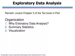
WHAT IS EDA? • The analysis of datasets based on various numerical methods and graphical tools. • Exploring data for patterns, trends, underlying structure, deviations from the trend, anomalies and strange structures. • It facilitates discovering unexpected as well as conforming the expected. • Another definition: An approach/philosophy for data analysis that employs a variety of techniques (mostly graphical).
AIM OF THE EDA • Maximize insight into a dataset • Uncover underlying structure • Extract important variables • Detect outliers and anomalies • Test underlying assumptions • Develop valid models • Determine optimal factor settings (Xs)
AIM OF THE EDA • The goal of EDA is to open-mindedly explore data. • Tukey: EDA is detective work… Unless detective finds the clues, judge or jury has nothing to consider. • Here, judge or jury is a confirmatory data analysis • Tukey: Confirmatory data analysis goes further, assessing the strengths of the evidence. • With EDA, we can examine data and try to understand the meaning of variables. What are the abbreviations stand for.
STEPS OF EDA • Generate good research questions • Data restructuring: You may need to make new variables from the existing ones. • Instead of using two variables, obtaining rates or percentages of them • Creating dummy variables for categorical variables • Based on the research questions, use appropriate graphical tools and obtain descriptive statistics. Try to understand the data structure, relationships, anomalies, unexpected behaviors. • Try to identify confounding variables, interaction relations and multicollinearity, if any. • Handle missing observations • Decide on the need of transformation (on response and/or explanatory variables). • Decide on the hypothesis based on your research questions
AFTER EDA • Confirmatory Data Analysis: Verify the hypothesis by statistical analysis • Get conclusions and present your results nicely.
Classification of EDA* • Exploratory data analysis is generally cross-classified in two ways. First, each method is either non-graphical or graphical. And second, each method is either univariate or multivariate (usually just bivariate). • Non-graphical methods generally involve calculation of summary statistics, while graphical methods obviously summarize the data in a diagrammatic or pictorial way. • Univariate methods look at one variable (data column) at a time, while multivariate methods look at two or more variables at a time to explore relationships. Usually our multivariate EDA will be bivariate (looking at exactly two variables), but occasionally it will involve three or more variables. • It is almost always a good idea to perform univariate EDA on each of the components of a multivariate EDA before performing the multivariate EDA. *Seltman, H.J. (2015). Experimental Design and Analysis. http://www.stat.cmu.edu/~hseltman/309/Book/Book.pdf
EXAMPLE 1 Data from the Places Rated Almanac *Boyer and Savageau, 1985) 9 variables fro 329 metropolitan areas in the USA • Climate mildness • Housing cost • Health care and environment • Crime • Transportation supply • Educational opportunities and effort • Arts and culture facilities • Recreational opportunities • Personal economic outlook + latitude and longitude of each city Questions: How is climate related to location? Are there clusters in the data (excluding location)? Are nearby cities similar? Any relation bw economic outlook and crime? What else???
EXAMPLE 2 • In a breast cancer research, main questions of interest might be • Does any treatment method result in a higher survival rate? Can a particular treatment be suggested to a woman with specific characteristic? • Is there any difference between patients in terms of survival rates (e.g. Are white woman more likely to survive compare the black woman if they are both at the same stage of disease?)
EXAMPLE 3 • In a project, investigating the well-being of teenagers after an economic hardship, main questions can be • Is there a positive ( and significant) effect of economic problems on distress? • Which other factors can be most related to the distress of teenagers? e.g. age, gender,…?
EXAMPLE 4* New cancer cases in the U.S. based on a cancer registry • The rows in the registry are called observations they correspond to individuals • The columns are variables or data fields they correspond to attributes of the individuals https://www.biostat.wisc.edu/~lindstro/2.EDA.9.10.pdf
Examples of Variables • Identifier(s): - patient number, - visit # or measurement date (if measured more than once) • Attributes at study start (baseline): - enrollment date, - demographics (age, BMI, etc.) - prior disease history, labs, etc. - assigned treatment or intervention group - outcome variable • Attributes measured at subsequent times - any variables that may change over time - outcome variable
Data Types and Measurement Scales • Variables may be one of several types, and have a defined set of valid values. • Two main classes of variables are: Continuous Variables: (Quantitative, numeric). Continuous data can be rounded or \binned to create categorical data. Categorical Variables: (Discrete, qualitative). Some categorical variables (e.g. counts) are sometimes treated as continuous.
Categorical Data • Unordered categorical data (nominal) 2 possible values (binary or dichotomous) Examples: gender, alive/dead, yes/no. Greater than 2 possible values - No order to categories Examples: marital status, religion, country of birth, race. • Ordered categorical data (ordinal) Ratings or preferences Cancer stage Quality of life scales, National Cancer Institute's NCI Common Toxicity Criteria (severity grades 1-5) Number of copies of a recessive gene (0, 1 or 2)
EDA Part 2: Summarizing Data With Tables and Plots Examine the entire data set using basic techniques before starting a formal statistical analysis. • Familiarizing yourself with the data. • Find possible errors and anomalies. • Examine the distribution of values for each variable.
Summarizing Variables • Categorical variables Frequency tables - how many observations in each category? Relative frequency table - percent in each category. Bar chart and other plots. • Continuous variables Bin the observations (create categories .e.g., (0-10), (11-20), etc.) then, treat as ordered categorical. Plots specific to Continuous variables. The goal for both categorical and continuous data is data reduction while preserving/extracting key information about the process under investigation.
Categorical Data Summaries Tables Cancer site is a variable taking 5 values • categorical or continuous? • ordered or unordered?
Frequency Table • Frequency Table: Categories with counts • Relative Frequency Table: Percentage in each category
Graphing a Frequency Table - Bar Chart: Plot the number of observations in each category:
Continuous Data - Tables Example: Ages of 10 adult leukemia patients: 35; 40; 52; 27; 31; 42; 43; 28; 50; 35 One option is to group these ages into decades and create a categorical age variable:
We can then create a frequency table for this new categorical age variable.
Continuous data - plots A histogram is a bar chart constructed using the frequencies or relative frequencies of a grouped (or \binned") continuous variable It discards some information (the exact values), retaining only the frequencies in each \bin"
Plotting Functions R has several distinct plotting systems Base R functions • hist() • barplot() • boxplot() • plot() lattice package ggplot2 package
Boxplot > boxplot(mtcars$mpg, main = "Miles per Gallon")
The boxplot function can also take a formula as an argument mpg cyl \mpg conditional on cyl" > boxplot(mpg ~ cyl, + data = mtcars, + main = "Miles per Gallon by Number of Cylinders", + xlab = "Cylinders", + ylab = "Miles per Gallon")
> # Expand the formula > boxplot(mpg ~ cyl + am, + data = mtcars, + main = "MPG by Number of Cylinders & Transmissions”)
Histogram Takes a vector, and plots the distribution of values > hist(mtcars$mpg)
Bar Chart Use the table function to create a two-way frequency table, and plotting options to group bars > counts <- table(mtcars$cyl, mtcars$am) > colnames(counts) <- c("Auto", "Manual") > barplot(counts, + main = "Number of Cars by Transmission and Cylinders", + xlab = "Transmission", + beside = TRUE, + legend = rownames(counts))
Scatterplot > plot(mtcars$mpg, + mtcars$hp, + xlab = "Miles per Gallon", + ylab = "Horsepower")
> # create a vector for conditional color coding > colorcode <- ifelse(mtcars$am == 0, "red", "blue") > plot(mtcars$mpg, + mtcars$hp, + xlab = "Miles per Gallon", + ylab = "Horsepower", + col = colorcode)
Lattice graphics* • lattice is an add-on package that implements Trellis graphics (originally developed for S and S-PLUS) in R. It is a powerful and elegant high-level data visualization system, with an emphasis on multivariate data. • To fix ideas, we start with a few simple examples. We use the Chem97 dataset from the mlmRev package. > library(mlmRev) > data(Chem97, package = "mlmRev") > head(Chem97) lea school student score gender age gcsescoregcsecnt 1 1 1 1 4 F 3 6.625 0.3393157 2 1 1 2 10 F -3 7.625 1.3393157 3 1 1 3 10 F -4 7.250 0.9643157 4 1 1 4 10 F -2 7.500 1.2143157 5 1 1 5 8 F -1 6.444 0.1583157 6 1 1 6 10 F 4 7.750 1.4643157 *All notes related to lattice graphics: https://www.isid.ac.in/~deepayan/R-tutorials/labs/04_lattice_lab.pdf
Lattice graphics • The dataset records information on students appearing in the 1997 A-level chemistry examination in Britain. • We are only interested in the following variables: • score: point score in the A-level exam, with six possible values (0, 2, 4, 6, 8). • gcsescore: average score in GCSE exams. This is a continuous score that may be used as a predictor of the A-level score. • gender: gender of the student. • Using lattice, we can draw a histogram of all the gcsescore values using > library(lattice) > histogram(~ gcsescore, data = Chem97)
Lattice graphics • histogram(~ gcsescore, data = Chem97) • This plot shows a reasonably symmetric unimodal distribution, but is otherwise uninteresting. A more interesting display would be one where the distribution of gcsescore is compared across different subgroups, say those defined by the A-level exam score.
Lattice graphics > histogram(~ gcsescore | factor(score), data = Chem97)
Lattice graphics • More effective comparison is enabled by direct superposition. This is hard to do with conventional histograms, but easier using kernel density estimates. In the following example, we use the same subgroups as before in the different panels, but additionally subdivide the gcsescore values by gender within each panel.
Lattice graphics > densityplot(~ gcsescore | factor(score), Chem97, groups = gender, plot.points = FALSE, auto.key = TRUE)
Lattice graphics • Several standard statistical graphics are intended to visualize the distribution of a continuous random variable. We have already seen histograms and density plots, which are both estimates of the probability density function. Another useful display is the normal Q-Q plot, which is related to the distribution function F(x) = P(X ≤ x). Normal Q-Q plots can be produced by the lattice function qqmath(). • Normal Q-Q plots plot empirical quantiles of the data against quantiles of the normal distribution (or some other theoretical distribution). They can be regarded as an estimate of the distribution function F, with the probability axis transformed by the normal quantile function. They are designed to detect departures from normality; for a good fit, the points lie approximate along a straight line. In the plot above, the systematic convexity suggests that the distributions are left-skewed, and the change in slopes suggests changing variance.
Lattice graphics > qqmath(~ gcsescore | factor(score), Chem97, groups = gender, + f.value = ppoints(100), auto.key = list(columns = 2), + type = c("p", "g"), aspect = "xy")
Lattice graphics The type argument adds a common reference grid to each panel that makes it easier to see the upward shift in gcsescore across panels. The aspect argument automatically computes an aspect ratio. Two-sample Q-Q plots compare quantiles of two samples (rather than one sample and a theoretical distribution). They can be produced by the lattice function qq(), with a formula that has two primary variables. In the formula y ~ x, y needs to be a factor with two levels, and the samples compared are the subsets of x for the two levels of y. For example, we can compare the distributions of gcsescore for males and females, conditioning on A-level score > qq(gender ~ gcsescore | factor(score), Chem97, + f.value = ppoints(100), type = c("p", "g"), aspect = 1)
The plot suggests that females do better than males in the GCSE exam for a given A-level score (in other words, males tend to improve more from the GCSE exam to the A-level exam), and also have smaller variance (except in the first panel).
Lattice graphics • A well-known graphical design that allows comparison between an arbitrary number of samples is the comparative box-and-whisker plot. • Box-and-whisker plots can be produced by the lattice function bwplot(). > bwplot(factor(score) ~ gcsescore | gender, Chem97)