Download
1 / 98
980 likes | 1.02k Views
Motion. ECE 847: Digital Image Processing. Stan Birchfield Clemson University. Outline. Motion basics Lucas-Kanade algorithm Horn-Schunck algorithm. What if you only had one eye?. Depth perception is possible by moving eye.

E N D
Motion ECE 847:Digital Image Processing Stan Birchfield Clemson University
Outline • Motion basics • Lucas-Kanade algorithm • Horn-Schunck algorithm
What if you only had one eye? Depth perception is possible by moving eye S. Birchfield, Clemson Univ., ECE 847, http://www.ces.clemson.edu/~stb/ece847
Head movements for depth perception Some animals move their heads to generate parallax pigeon praying mantis http://pinknpurplelizard.files.wordpress.com/2008/06/pigeon1.jpg http://www.animalwebguide.com/Praying-Mantis.htm S. Birchfield, Clemson Univ., ECE 847, http://www.ces.clemson.edu/~stb/ece847
Parallax Motion parallax – apparent displacement of object viewed along two different lines of sight http://www.infovis.net/imagenes/T1_N144_A6_DifMotion.gif S. Birchfield, Clemson Univ., ECE 847, http://www.ces.clemson.edu/~stb/ece847
Difference between stereo and 2-frame motion • Stereo: • Images taken at same time • Scene is guaranteed to be static • Epipolar constraint restricts search to 1D • 2-frame motion: • Images taken at different times • Objects in scene may have independently moved • Epipolar constraint no longer guaranteed Of course, motion involves a video sequence of images S. Birchfield, Clemson Univ., ECE 847, http://www.ces.clemson.edu/~stb/ece847
Motion field and optical flow • Motion field – The actual 3D motion projected onto image plane • Optical flow – The “apparent” motion of the brightness pattern in an image(sometimes called optic flow) S. Birchfield, Clemson Univ., ECE 847, http://www.ces.clemson.edu/~stb/ece847
When are the two different? Barber pole illusion Television / movie (no motion field) Rotating ping-pong ball http://homepages.inf.ed.ac.uk/rbf/CVonline/LOCAL_COPIES/OWENS/LECT12/node4.html (no optical flow) S. Birchfield, Clemson Univ., ECE 847, http://www.ces.clemson.edu/~stb/ece847
Perhaps an aperture problem discussed later. Optical flow breakdown * From Marc Pollefeys COMP 256 2003
Another illusion from G. Bradski, CS223B
Motion field Point in world: Projection onto image: dp/dt p Motion of point in world: dx/dt camera translation rotation where S. Birchfield, Clemson Univ., ECE 847, http://www.ces.clemson.edu/~stb/ece847
Motion field (cont.) Image velocity of projection: dp/dt p Expanding yields: dx/dt camera Note that rotation gives no depth information depth S. Birchfield, Clemson Univ., ECE 847, http://www.ces.clemson.edu/~stb/ece847
Motion field (cont.) Two special cases: Note: This is a radial field emanating from the instantaneous epipole Note: Here the instantaneous epipole is at infinity S. Birchfield, Clemson Univ., ECE 847, http://www.ces.clemson.edu/~stb/ece847
Optical Flow Assumptions:Brightness Constancy * Slide from Michael Black, CS143 2003
Optical Flow Assumptions: * Slide from Michael Black, CS143 2003
Optical Flow Assumptions: * Slide from Michael Black, CS143 2003
Optical flow constraint equation Brightness constancy assumption velocity (to be estimated) pixel Optical flow constraint equation image image velocity(unknown) image gradient(known) temporal derivative(known) S. Birchfield, Clemson Univ., ECE 847, http://www.ces.clemson.edu/~stb/ece847
Recall: Taylor series A function f(x) can be approximated near x=x0 by Linear approximation is If f is a function of 2 variables: If f is a function of 3 variables: S. Birchfield, Clemson Univ., ECE 847, http://www.ces.clemson.edu/~stb/ece847
Deriving the optical flow constraint equation Image at time t Image at time t + Dt Brightness constancy assumption: Taylor series expansion: Putting together yields: S. Birchfield, Clemson Univ., ECE 847, http://www.ces.clemson.edu/~stb/ece847
Deriving the optical flow constraint equation From previous slide: Divide both sides by Dt and take the limit: or optical flow constraint equation More compactly, S. Birchfield, Clemson Univ., ECE 847, http://www.ces.clemson.edu/~stb/ece847
Aperture problem From previous slide: Key idea: Any function looks linear through small `aperture’ This is one equation, two unknowns! (Underconstrained problem) true motion gradient another possible answer I(x,y,t+Dt)=x isophote I(x,y,t)=xisophote We can only compute component of motion in direction of gradient: S. Birchfield, Clemson Univ., ECE 847, http://www.ces.clemson.edu/~stb/ece847
Aperture Problem Exposed Motion along just an edge is ambiguous from G. Bradski, CS223B
Two approaches to overcome aperture problem • Horn-Schunck (1980) • Assume neighboring pixels are similar • Add regularization term to enforce smoothness • Compute (u,v) for every pixel in image • Dense optical flow • Lucas-Kanade (1981) • Assume neighboring pixels are same • Use additional equations to solve for motion of pixel • Compute (u,v) for a small number of pixels (features); each feature treated independently of other features • Sparse optical flow S. Birchfield, Clemson Univ., ECE 847, http://www.ces.clemson.edu/~stb/ece847
Outline • Motion basics • Lucas-Kanade algorithm • Horn-Schunck algorithm
Lucas-Kanade Recall scalar “equation” was derived by linearizing function about current estimate: + higher order terms Total displacement that we want (u) Reinterpret: Incremental displacement that we can compute (uD) This is one iteration of Newton’s method. So we iterate and accumulate: Initial estimate (could be zero) S. Birchfield, Clemson Univ., ECE 847, http://www.ces.clemson.edu/~stb/ece847
Recall: Newton’s method Goal: Find root (or zero) of functionf(x) • Use first-order approximation(tangent line) • Start with initial guess • Iterate: • Use derivative to find root, under assumption that function is linear • Result used as estimate for next iteration y f’(x0) f(x0) Dy x Dx x1 x0 Solution: Iterate x = x1 = x0 + Dx S. Birchfield, Clemson Univ., ECE 847, http://www.ces.clemson.edu/~stb/ece847
Recall: Newton’s method Goal: Find root (or zero) of functionf(x) • Use first-order approximation(tangent line) • Start with initial guess • Iterate: • Use derivative to find root, under assumption that function is linear • Result used as estimate for next iteration y f’(x1) f(x1) Dy x x2 x1 Dx Solution: Iterate x = x2 = x1 + Dx S. Birchfield, Clemson Univ., ECE 847, http://www.ces.clemson.edu/~stb/ece847
Recall: Newton’s method Goal: Find extremum (min or max) of functionf(x) Key idea: Extremum occurs when f’(x)=0 Replace f with f’ Solution: Iterate Note: Now we need 2nd derivative S. Birchfield, Clemson Univ., ECE 847, http://www.ces.clemson.edu/~stb/ece847
Recall: Gauss-Newton method Goal: Find extremum (min or max) of functionf(x)=( e(x) )2 Key idea: When f(x) has this special form, derivatives of f are easy to compute: f’(x) = 2 e(x) e’(x) f”(x) = 2 ( e’(x) )2 + 2 e(x) e”(x) Ignoring the 2nd derivative yields f”(x) ≈ 2 ( e’(x) )2 Solution: Iterate Note: Now we only need 1st derivative S. Birchfield, Clemson Univ., ECE 847, http://www.ces.clemson.edu/~stb/ece847
1D Lucas-Kanade tracking 2D: 1D: Ix Spatial derivative uD I(x) J(x) It Temporal derivative x Incremental displacement: S. Birchfield, Clemson Univ., ECE 847, http://www.ces.clemson.edu/~stb/ece847
1D Lucas-Kanade tracking First iteration: Given two images, and position x I(x) J(x) x S. Birchfield, Clemson Univ., ECE 847, http://www.ces.clemson.edu/~stb/ece847
1D Lucas-Kanade tracking First iteration: Compute temporal derivative I(x) J(x) It(1)=J(x)-I(x) Temporal derivative x S. Birchfield, Clemson Univ., ECE 847, http://www.ces.clemson.edu/~stb/ece847
1D Lucas-Kanade tracking First iteration: Compute spatial derivative Ix=dI/dx Spatial derivative I(x) J(x) It(1)=J(x)-I(x) Temporal derivative x S. Birchfield, Clemson Univ., ECE 847, http://www.ces.clemson.edu/~stb/ece847
1D Lucas-Kanade tracking First iteration: Compute incremental displacement Ix=dI/dx Spatial derivative uD(1) I(x) J(x) It(1)=J(x)-I(x) Temporal derivative x Total displacement: Compute incremental displacement: S. Birchfield, Clemson Univ., ECE 847, http://www.ces.clemson.edu/~stb/ece847
1D Lucas-Kanade tracking First iteration: Shift I(x) to the right by uD … or Ix=dI/dx Spatial derivative uD(1) I(x-u) J(x) It(1)=J(x)-I(x) Temporal derivative x Total displacement: Compute incremental displacement: S. Birchfield, Clemson Univ., ECE 847, http://www.ces.clemson.edu/~stb/ece847
1D Lucas-Kanade tracking First iteration: Shift J(x) to the left by uD (equivalent) Ix=dI/dx Spatial derivative uD(1) I(x) J(x+u) It(1)=J(x)-I(x) Temporal derivative x Total displacement: Compute incremental displacement: S. Birchfield, Clemson Univ., ECE 847, http://www.ces.clemson.edu/~stb/ece847
1D Lucas-Kanade tracking Second iteration: Repeat same steps Ix=dI/dx Spatial derivative(can reuse this) uD(2) I(x) J(x+u) It(2)=J(x)-I(x) Temporal derivative x Total displacement: Compute incremental displacement: S. Birchfield, Clemson Univ., ECE 847, http://www.ces.clemson.edu/~stb/ece847
1D Lucas-Kanade tracking … until convergence I(x) J(x+u) x Total displacement: S. Birchfield, Clemson Univ., ECE 847, http://www.ces.clemson.edu/~stb/ece847
2D Lucas-Kanade in a nutshell 2D: 1D: Instead of solving for uDwe need to solve for uD=(uD,vD) Given two consecutive images I and J from a sequence, • Take pixel-wise difference between them It • Compute gradient of one image Ix and Iy • Sum over window to get Z and e • Solve ZuD=e for uD • Update u=uD(1)+... • Shift image • Repeat (2x2 matrix) (2x1 vector) What are Z and e? Why do we need to sum over window? S. Birchfield, Clemson Univ., ECE 847, http://www.ces.clemson.edu/~stb/ece847
Lucas-Kanade derivation Scalar equation with two unknowns is an underconstrained system: Introduce constraint. Assume neighboring pixels have samemotion: window around pixel n = number of pixels in window or Can solve this directly using least squares, or (better yet) … S. Birchfield, Clemson Univ., ECE 847, http://www.ces.clemson.edu/~stb/ece847
Lucas-Kanade derivation Multiply by AT : or or (2x2 matrix) (2x1 vector) (region of neighboring pixels) S. Birchfield, Clemson Univ., ECE 847, http://www.ces.clemson.edu/~stb/ece847
RGB version of Lucas-Kanade • For color images, we can get more equations by using all color channels • E.g., for 7x7 window we have 49*3=147 equations! • But color channels are highly correlated, so rarely helps much S. Birchfield, Clemson Univ., ECE 847, http://www.ces.clemson.edu/~stb/ece847
Lucas-Kanade pseudocode Typically R is a pixel x=(x,y) and the width of the square window OK to move this out of loop S. Birchfield, Clemson Univ., ECE 847, http://www.ces.clemson.edu/~stb/ece847
can x and y be floats? can x and y be floats? (solving 2x2 equation is easy: invert Z by hand) S. Birchfield, Clemson Univ., ECE 847, http://www.ces.clemson.edu/~stb/ece847
Lucas-Kanade details Need to • loop over frames and features • interpolate • declare features lost • detect good features • smooth the image to handle large motions S. Birchfield, Clemson Univ., ECE 847, http://www.ces.clemson.edu/~stb/ece847
1. Loop over frames and features • We have only described the procedure for • a single pixel (using its surrounding window) • two consecutive image frames • Need to wrap this in 2 for loops • over frames in the sequence • over features (sparse pixels) in the image S. Birchfield, Clemson Univ., ECE 847, http://www.ces.clemson.edu/~stb/ece847
Loop over frames and features features is 2D array over features and frames float colon selects entire row (like Matlab) float float (Conceptually) constructs a region from pixel and window-width (In reality) does nothing; just pass both parameters to LucasKanade S. Birchfield, Clemson Univ., ECE 847, http://www.ces.clemson.edu/~stb/ece847
2. Interpolate • After very first iteration, x and y can be floats; same for u and v • Could simply round to nearest integer before computing • But results are more accurate if we interpolate S. Birchfield, Clemson Univ., ECE 847, http://www.ces.clemson.edu/~stb/ece847
Linear interpolation f(x0+2) f(x0-1) f(x0) f(x0+1) 1D function x0-1 x0 x x0+1 x0+2 0≤a<1 f(x) ≈ f(x0) + (x-x0) ( f(x0+1) – f(x0) ) = f(x0) + a ( f(x0+1) – f(x0) ) = (1 –a) f(x0) + a f(x0+1) S. Birchfield, Clemson Univ., ECE 847, http://www.ces.clemson.edu/~stb/ece847
Bilinear interpolation x0-1 x0 x x0+1 x0+2 2D function y0-1 a Note: These are the pixel squares f00 f10 y0 b y y0+1 f01 f11 y0+2 f(x0,y) ≈ (1-b)f00 + bf01 f(x0+1,y) ≈ (1-b)f10 + bf11 f(x,y) ≈ (1-a) [(1-b)f00 + bf01] + a[(1-b)f10 + bf11] = (1-a)(1-b)f00 + (1-a)bf01 + a(1-b)f10 + abf11 S. Birchfield, Clemson Univ., ECE 847, http://www.ces.clemson.edu/~stb/ece847