Download
1 / 33
410 likes | 669 Views
Abyssal Circulation. Deep ocean is below the permanent thermocline (at 1~km) with ~2 o - 4 o C below 2 km (0 o -2 o C at 4 km typically). Waters of such low temperatures can only be formed by cooling in Polar Regions.

E N D
Abyssal Circulation Deep ocean is below the permanent thermocline (at 1~km) with ~2o-4oC below 2 km (0o-2oC at 4 km typically). Waters of such low temperatures can only be formed by cooling in Polar Regions. In both Polar Regions the zones of sinking are quite narrow, and the convective sinking itself is difficult to observe directly. The sinking instead is largely inferred from the distribution of ocean properties such as temperature, salinity, and especially oxygen. The deep water from the major sources is between 10-20 Sv, with a considerable fraction estimated to be water entrained during the sinking as well as entrained laterally as the source water into the deep ocean. The presence at other latitudes of such cold water implies a large scale deep circulation, the abyssal circulation, which carries the cold water formed in Polar Regions to fill the rest of the deep ocean basins. The water must eventually rise to the surface and, heated to the observed surface temperatures, must then flow poleward to replace the water which has sunk to the bottom, forming an endless global cell of motion.
The process of deep water circulation Although the origins and characteristics of the deep water are reasonably well known, much less is known about the processes by which the water comes to fill the deep ocean. Is it by deep underwater currents such as we have in the surface ocean, or is it by some slow mixing and diffusion process in which heat and salt are being transferred by eddy diffusion with no net transfer of mass? Both processes are important, but the relative role of each has yet to be sorted out. (Knauss, p180-181) It has been suggested that most north-south advection is by the deep western boundary currents and that most east-west movement in the deep water is by turbulent diffusion. It remains to be seen whether such a hypothesis is substantiated. One problem with the development of any theory of deep circulation is that we have little direct evidence of where the water returns to the surface. The sources of deep water are few and are known. However, the water that sinks from the surface must be replaced. It is not known whether the primary mechanism of return is limited to a few locations, such as regions of upwelling, or whether most of the water returns slowly over such a wide area that it cannot be detected. (Knauss, p182-183)
FIGURE S7.40 (From Talley et al. 2011) The role of vertical (diapycnal) diffusion in the MOC, replacing Sandström's (1908) deep tropical warm source with diapycnal diffusion that reaches below the effect of high latitude cooling.
FIGURE 9.15(a) Schematics of deep circulation. (a) NSOW (blue), LSW (white dashed), and upper ocean (red, orange, and yellow) in the northern North Atlantic. Source: From Schott and Brandt (2007). (From Talley et al. 2011)
FIGURE 9.15(b) (From Talley et al. 2011) Schematics of deep circulation. (b) Deep circulation pathways emphasizing DWBCs (solid) and their recirculations (dashed). Red: NSOW. Brown: NADW. Blue: AABW. This figure can also be found in the color insert. (M.S. McCartney, personal communication, 2009.)
Dynamical Model of the Abyssal Flow A conceptual framework of the abyssal circulation was developed by Stommel (1958) and Stommel and Arons (1960a,b), which explains dynamically the horizontal structure of the vertically averaged abyssal circulation, especially its western boundary currents. The theory is actually a straightforward application of the Sverdrup theory. • Assumptions: • In compensation for the known sinking of the near surface water in small regions, there is a general slow upward movement of deep water over most of the rest of the ocean. • The mean horizontal deep flow in the open ocean is strictly geostrophic, in the sense that the streamlines parallel isobars, and their speeds inversely proportional to their spacing and to the sine of the latitude.
From assumption (1) The slow global upward advection of cold water from abyss balances the downward diffusion of heat from the upper layer at the bottom of the main thermocline: or where is the upwelling velocity of the abyssal water at the base of thermocline is the downward heat flux. This leads to an estimate of vertical velocity at the base of the thermocline as: where d is the vertical scale of variations of the heat flux. On the other hand, since the overall area of the world oceans is toughly , to obtain a flux of 20 Sv from the abyss to the thermocline to replace the waters sinking into the abyss in the Polar Regions, an independent estimate of the upwelling is For a vertical scale d of the order of 1 km, this would suggest ~0.66 cm2/s. This is larger than direct measurement of 0.11 cm2/s (Ledwell et al., 1993). (The estimate of transport (20 Sv) may be too high)
From assumption (2) The geostrophic vorticity balance within the deep ocean then is • Integrating the vorticity equation vertically from the ocean bottom to the “top” of the deep water, we have where is the total meridional transport of the abyssal circulation. • wB is the vertical velocity at the bottom. If we take the floor of the ocean to be level in the large scale mean, wB is zero. Then we have the “Sverdrup” relation in the seep ocean Since wis everywhere positive except for the very limited areas in the polar regions, V>0 in the northern hemisphere and V<0 in the southern hemisphere. The interior transport is toward the sources. A western boundary is required to close the mass balance.
FIGURE S7.41 (a) Abyssal circulation model. After Stommel and Arons (1960a). (b) Laboratory experiment results looking down from the top on a tank rotating counterclockwise around the apex (So) with a bottom that slopes towards the apex. There is a point source of water at So. The dye release in subsequent photos shows the Deep Western Boundary Current, and flow in the interior Si beginning to fill in and move towards So. Source: From Stommel, Arons, & Faller (1958). (From Talley et al. 2011)
Stommel, Arons and Faller Experiment
Stommel-Arons Theory: Abyssal Flow on a Sphere In spherical coordinates, considera latitudinal bounded two-layer ocean. Local sinking S0 is specified at pole from the upper to lower layer. The return flow has a vertical velocity wo, specified over the area of the ocean basin at the top of the abyssal layer. For the layer representing the abyss, the motion is geostrophic. , where R is radius of the earth and and are longitude and latitude. The continuity equator is .
Combining the geostrophic and continuity equations, we derive the Sverdrup vorticity equation with and Integrating vertically over the depth H yields: or • v is always poleward as long as wo is positive. • v must vanish at the equator. • Cross equatorial flow must be in regions where the Sverdrup balance is broken (i.e., the western boundary). From , we have and Assume wo is independent of horizontal position (constant), we have .
Consider an ocean basin from the equator to the pole. For an arbitrary latitude , the sum of the interior flux (TI) and the western boundary current’s transport (Tw) through an arbitrary latitude is balanced by the source’s contribution So and flux out of the abyss through the interface to the north of (Tout). i.e., Since . If the mass is balanced over the northern hemisphere In this case,
Discussion of the results: • The western boundary layer transport is southward for all ≥0. • The boundary transport is exactly twice the source strength at the pole since the boundary current must carry southward the fluid issuing from the source as well as all of the impinging interior flow. • The interior flow comprises a basinwide recirculation and has a northward mass flux at the apex equal to the source strength. • Half the mass flux of the boundary layer comes from the source and half from the recirculating interior flow. • The interior is fed from the western boundary current as the current flows southward, which falls to zero as it approaches the equator. During the southward movement, the western boundary current loses a total mass flux equal to 2So. • One half of this flow is recirculated in the interior and ends up at the apex to return through the western boundary current. • The other half is lost through the interface to the thermocline and is directly replaced in the western boundary layer at the apex by the source.
Mass Transport in Layers FIGURE 14.5 (from Talley et al. 2011, DPO) Meridional overturning circulation transport calculation: example for four layers. The mass transports for each layer “i” through the southern and northern boundaries of each layer are VSi and VNi. The vertical transport across each interface is Wi. Arrow directions are those for positive sign; the actual transports can be of any magnitude and sign. The sum of the four transports (two horizontal and two vertical) into a given closed layer must be 0 Sv. The small amount of transport across the sea surface due to evaporation and precipitation is not depicted.
Other Major Water Masses Antarctic Circumpolar Water (CPW) Below the surface and extending to the bottom at depths to 4000m. Maximum temperature is 1.5-2.5oC at 300-600m and then decreases to between 0o-0.5oC near the bottom. Salinity 34.7psu. Carried around by Antarctic Circumpolar Current (ACC) and found all around the continent at about the same depth (CPW is probably a mixture of Antarctic Bottom Water and the North Atlantic Deep Water). Antarctic Intermediate Water (AAIW) Formed by the sinking of the Antarctic surface water, mostly from convection east of southern Chile and west of southern Argentina. It is also suggested that the AIW formation occurs circumpolarly by cross-polar-front mixing between low-salinity surface water and subantarctic surface water. AIW is quite homogeneous (T=2o-3oC, S=34.2) and has density t=27.4 higher than the water further north. It spreads into all oceans with the Circumpolar Current and continues northward below the surface. It has a thickness of 500 m and forms a tongue of relatively low salinity water with core at 800 to 1000 m at 40oS. AIW mixes with more saline water from above and below during northward movement. (Intermediate Water may also be formed in the northern hemisphere by convection or subduction.)
A Cross Section along the Western Atlantic Ocean Antarctic Intermediate Water North Atlantic Deep Water Antarctic Bottom Water Note the minimum in , which seems to imply a vertical instability. However, it is because is not adequate. In fact, using 4 gets stable stratification.
A series of TS-diagrams from the Atlantic Ocean, from 40°S to 40°N, showing the erosion of the salinity minimum associated with Antarctic Intermediate Water along the path of the water mass. The red line traces the salinity minimum produced by the relatively fresh Antarctic Intermediate Water. Color indicates oxygen content. Note how the oxygen content associated with the salinity minimum decreases from south to north, indicating the aging of the Antarctic Intermediate Water. (based on OceanAtlas of J. Osborne, J. Swift and E. P. Flinchem) From M. Tomczak: Introduction to Physical Oceanography http://gaea.es.flinders.edu.au/~mattom/IntroOc/lecture07.html
FIGURE 9.16(a-d) Salinity and meridional transport in isopycnal layers at (a, b) 24°N in 1981 and (c, d) 32°S in 1959/1972. The inset map shows section locations. The isopycnals (σθ, σ2, σ4) that define the layers are contoured in black on the salinity sections. Figures 9.16a, c can also be found in the color insert. See also online supplementary Figures S9.24 and S9.25 for examples from Bryden, Longworth, and Cunningham (2005b) and Ganachaud (2003). After Talley (2008), based on Reid (1994) velocities. (From Talley et al. 2011)
Sketch of the water mass distribution in the world ocean AABW: Antarctic Bottom Water, CPW: Circumpolar Water, NADW: North Atlantic Deep Water, PDW: Pacific Deep Water, AAIW: Antarctic Intermediate Water, AIW: Arctic Intermediate Water, MedW: Mediterranean Water, RedSW: Red Sea Water, gold: Central Water, brown: surface water. From M. Tomczak: Introduction to Physical Oceanography http://gaea.es.flinders.edu.au/~mattom/IntroOc/lecture07.html
Pacific Deep Water The distribution of oxygen (Figure 9.4c) indicates the penetration of AABW into thenorthern hemisphere below 3000 m and active circulation associated with the spreading ofIntermediate Water above 1000 m depth. In the northern hemisphere, water in the depthrange 1000 - 3000 m does not participate much in the circulation; its properties are determined nearly entirely through slow mixing processes. This water is usually called PacificDeep Water (PDW), in analogy to the North Atlantic and Indian Deep Waters which occupythe same depth range. Oldest water > 1000 yrs Pacific Deep Water Uniform property in 2000-3000 m Old water type (about 1000 years) A mixture of AABW, NADW and AAIW No deep water formation in the North Pacific (Bering strait too shallow, North Atlantic water too fresh).
Figure 9.5 compares Deep Water properties of the three oceans. The different characterof Atlantic, Indian, and Pacific Deep Water comes out clearly. North Atlantic Deep Water isformed at the surface in a region of very high surface salinity and is therefore seen in the T-S diagram as a salinity maximum between Bottom and Intermediate Water. The Indian Deep Water is essentially the NADW advected into the Indian Ocean. In the T-S diagram it is present as a salinity maximum, with T-S values veryclose to those of NADW east of 40oE, the maximum being erodedfurther east and north through mixing with the waters above and below. In contrast, the T-S values of Pacific DeepWater do not depart very much from the mixing line between Bottom and IntermediateWater except in the vicinity of the Southern Ocean, where a faint salinity maximumindicates that traces of North Atlantic Deep Water, having crossed the Indian Ocean underthe name of Indian Deep Water, are entering the Pacific Ocean from the Great AustralianBight. It is thus seen that the constituents of Pacific Deep Water are Antarctic BottomWater, North Atlantic Deep Water, and Antarctic Intermediate Water. This mixing processconstitutes the common formation history of all Pacific Deep Water.
FIGURE 14.6(From Talley et al. 2011) Net transports (Sv) in isopycnal layers across closed hydrographic sections (1 Sv = 1 × 10⁶ m3/sec). (a) Three calculations from different sources are superimposed, each using three isopycnal layers (see header). Circles between sections indicate upwelling (arrow head) and downwelling (arrow tail) into and out of the layer defined by the circle color. Source: From Maltrud and McClean (2005), combining results from their POP model run, Ganachaud and Wunsch (2000), and Schmitz (1995).(b) Fourth calculation based on velocities from Reid (1994, 1997, 2003), with ribbons indicating flow direction and oveturn locations schematically. Source: From Talley (2008).
Deep water • Deep water is transported southward through the length of Atlantic and southward out of Pacific • Deep transport in the Indian Ocean is small and northward • Bottom water moves northward from the Antarctic into all three oceans
FIGURE 14.7 (from Talley et al. 2011) Modeled upwelling across the isopycnal 27.625 kg/m3, which represents upwelling from the NADW layer. This figure can also be found in the color insert. Source: From Kuhlbrodt et al. (2007); adapted from Döös and Coward (1997).
FIGURE 14.8 Meridional overturning streamfunction (Sv) from a high resolution general circulation model for the (a) Atlantic, (b) Pacific plus Indian, and (c) Indian north of the ITF. The Southern Ocean is not included. Source: From Maltrud and McClean (2005).
FIGURE 14.10(From Talley et al. 2011) Simplified global NADW cell, which retains sinking only somewhere adjacent to the northern North Atlantic and upwelling only in the Indian and Pacific Oceans. See text for usefulness of, and also issues with, this popularization of the global circulation, which does not include any Southern Ocean processes. Source: After Broecker (1987).
FIGURE 14.11(a) (From Talley et al. 2011) Global overturning circulation schematics. (a) The NADW and AABW global cells and the NPIW cell. See Figure S14.1 on the textbook Web site for a complete set of diagrams. This figure can also be found in the color insert. Source: From Talley (2011).
FIGURE 14.11(bc) (From Talley et al. 2011) Globaloverturningcirculationschematics. (b) Overturnfrom a SouthernOceanperspective. Source: AfterGordon (1991), Schmitz (1996b), and Lumpkin and Speer (2007). (c) Two-dimensionalschematicoftheinterconnected NADW, IDW, PDW, and AABW cells. Theschematics do not accuratelydepictlocationsofsinkingorthebroadgeographicscaleofupwelling. Colors: surfacewater (purple), intermediate and SouthernOcean mode water (red), PDW/IDW/UCDW (orange), NADW (green), AABW (blue). SeeFigure S14.1 on thetextbook Web sitefor a complete set ofdiagrams. Thisfigurecanalsobefound in thecolor insert. Source: FromTalley (2011).