Download
1 / 12
120 likes | 239 Views
Part I of the Fundamental Theorem says that we can use antiderivatives to compute definite integrals. Part II turns this relationship around: It tells us that we can use the definite integral to construct antiderivatives.

E N D
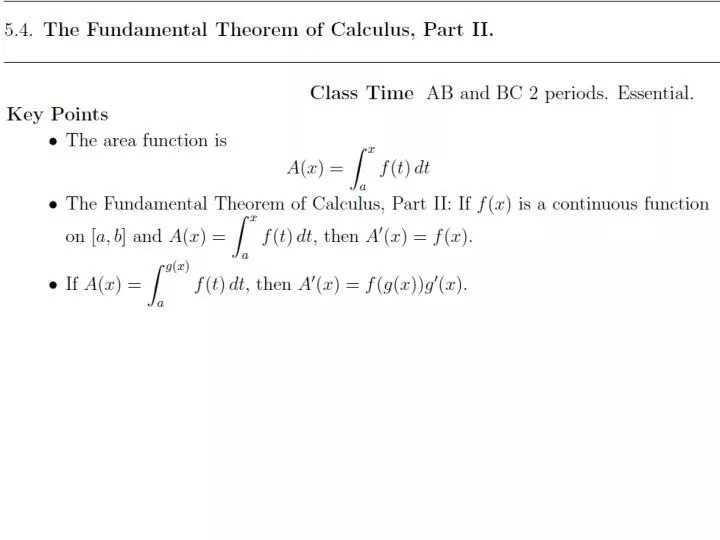
Part I of the Fundamental Theorem says that we can use antiderivatives to compute definite integrals. Part II turns this relationship around: It tells us that we can use the definite integral to constructantiderivatives. To state Part II, we introduce the area functionof f with lower limit a: In essence, we turn the definite integral into a function by treating the upper limit x as a variable.
THEOREM 1 Fundamental Theorem of Calculus, Part II Assume that f (x) is continuous on an open intervalI and let aI. Then the area function Equivalently, is an antiderivativeof f (x) on I; that is Furthermore, A (x) satisfies the initial condition A (a) = 0.
CONCEPTUAL INSIGHT Many applications (in the sciences, engineering, and statistics) involve functions for which there is no explicit formula. Often, however, these functions can be expressed as definite integrals (or as infinite series). This enables us to compute their values numerically and create plots using a computer algebra system. Figure 5 shows a computer-generated graph of an antiderivativeof f (x) = sin(x2), for which there is no explicit formula. Figure 5 Computer-generated graph of
Antiderivative as an Integral Let F (x) be the particular antiderivative of f (x) = sin (x2) satisfying THEOREM 1 Fundamental Theorem of Calculus, Part II Assume that f (x) is continuous on an open intervalI and let aI. Then the area function Equivalently, is an antiderivativeof f (x) on I; that is Furthermore, A (x) satisfies the initial condition A (a) = 0.
Differentiating an IntegralFind the derivative of THEOREM 1 Fundamental Theorem of Calculus, Part II Assume that f (x) is continuous on an open intervalI and let aI. Then the area function Equivalently, is an antiderivativeof f (x) on I; that is Furthermore, A (x) satisfies the initial condition A (a) = 0.
CONCEPTUAL INSIGHTThe FTC shows that integration and differentiation are inverse operations. By FTC II, if you start with a continuous function f (x) and form the integral then you get back the original function by differentiating: On the other hand, by FTC I, if you differentiate first and then integrate, you also recover f (x) [but only up to a constant f (a)]:
When the upper limit of the integral is a function of x rather than x itself, we use FTC II together with the Chain Rule to differentiate the integral. Find the derivative of
GRAPHICAL INSIGHT FTC II tells us that A (x) = f (x), or, in other words, f (x) is the rate of change of A (x). If we did not know this result, we might come to suspect it by comparing the graphs of A (x) and f (x). Consider the following: Figure 6 shows that the increase in area ΔA for a given Δx is larger at x2 than at x1 because f (x2) > f (x1). So the size of f (x) determines how quickly A (x) changes, as we would expect if A (x) = f (x).
GRAPHICAL INSIGHT FTC II tells us that A (x) = f (x), or, in other words, f (x) is the rate of change of A (x). If we did not know this result, we might come to suspect it by comparing the graphs of A (x) and f (x). Consider the following: Figure 7 shows that the sign of f (x) determines whether A (x) is increasing or decreasing. If f (x) > 0, then A (x) is increasing because positive area is added as we move to the right. When f (x) turns negative, A (x) begins to decrease because we start adding negative area. A (x) has a local max at points where f (x) changes sign from + to − (the points where the area turns negative), and has a local min when f (x) changes from − to +. This agrees with the First Derivative Test. These observations show that f (x) “behaves” like A (x), as claimed by FTC II.